Case study
Last updated on 2023-01-24 | Edit this page
Estimated time 122 minutes
Overview
Questions
- How do I analyse peptide count data in
R?
Objectives
- Demonstrate some ways of analysing NGS peptide count data
See the answers to each question for solutions.
Peptide count data
To round things out, we’ll explore some simulated peptide library data using what we’ve learned so far. Please follow along in an R markdown notebook on your own computer. The data is included in the data files you downloaded at the start of the course.
In this dataset, we’ve made an imaginary peptide insertion in the cap gene of AAV to create a plasmid library. We’ve then packaged this to create a vector library, and done a selection in some imaginary cells. We’ve therefore got data from plasmid, vector, DNA/entry and cDNA/expression libraries.
Imagine you’ve already done the counting using the counting pipeline, and now you want to explore the results.
You’ll start with four files, one for each library, each containing two columns: peptide and count. These files are called counts_plasmid.tsv, counts_vector.tsv, counts_entry.tsv, counts_expression.tsv.
The data here is simulated, so don’t interpret the results! If you want to see how I simulated the data, you can check it out on github.
Excercies
OUTPUT
── Attaching packages ─────────────────────────────────────── tidyverse 1.3.2 ──
✔ ggplot2 3.4.0      ✔ purrr   1.0.1
✔ tibble  3.1.8      ✔ dplyr   1.0.10
✔ tidyr   1.2.1      ✔ stringr 1.4.1
✔ readr   2.1.3      ✔ forcats 0.5.2
── Conflicts ────────────────────────────────────────── tidyverse_conflicts() ──
✖ dplyr::filter() masks stats::filter()
✖ dplyr::lag()    masks stats::lag()
R
# file paths
files <- here::here("episodes", "data", c("counts_plasmid.tsv",
                                          "counts_entry.tsv",
                                          "counts_expression.tsv",
                                          "counts_vector.tsv"))

# load data
counts <- read_tsv(files, col_types = "ci", id="file")

# create extra column
counts <- counts %>%
  mutate(lib = stringr::str_extract(file, "plasmid|vector|entry|expression")) %>%
  select(-file)

glimpse(counts)
OUTPUT
Rows: 40,000
Columns: 3
$ peptide <chr> "KGEWPFI", "SILPAEY", "EGSLHTV", "MYNQSEE", "HYMWLTD", "WNCCNI…
$ count   <int> 4, 3, 2, 1, 4, 3, 5, 7, 3, 2, 1, 2, 4, 6, 2, 5, 3, 2, 1, 6, 3,…
$ lib <chr> "plasmid", "plasmid", "plasmid", "plasmid", "plasmid", "plasmi…R
counts %>%
  group_by(lib) %>%
  summarise(n_pept = n_distinct(peptide),
            mean_count = mean(count),
            median_count = median(count),
            sd_count = sd(count),
            lib_size = sum(count))
OUTPUT
# A tibble: 4 × 6
  lib        n_pept mean_count median_count sd_count lib_size
  <chr>       <int>      <dbl>        <dbl>    <dbl>    <int>
1 entry       10000       3.18            2     6.18    31775
2 expression  10000       2.24            1     9.56    22367
3 plasmid     10000       3.98            3     3.00    39796
4 vector 10000 4.76 3 4.95 47553R
counts %>%
  group_by(lib) %>%
  slice_max(order_by=count, n=10)
OUTPUT
# A tibble: 43 × 3
# Groups:   lib [4]
   peptide count lib
   <chr>   <int> <chr>
 1 DSGFDYR   173 entry
 2 YYRVNEQ   139 entry
 3 TKIVCQG   130 entry
 4 PHGMDPM   112 entry
 5 EKMPHRS   101 entry
 6 PSFVTLG    87 entry
 7 TQCNAIG    87 entry
 8 GMEVEPY    85 entry
 9 AALHTQL    83 entry
10 NCAPHKG    76 entry
# … with 33 more rowsR
counts <- counts %>%
  group_by(lib) %>%
  mutate(frac = count/sum(count))

glimpse(counts)
OUTPUT
Rows: 40,000
Columns: 4
Groups: lib [4]
$ peptide <chr> "KGEWPFI", "SILPAEY", "EGSLHTV", "MYNQSEE", "HYMWLTD", "WNCCNI…
$ count   <int> 4, 3, 2, 1, 4, 3, 5, 7, 3, 2, 1, 2, 4, 6, 2, 5, 3, 2, 1, 6, 3,…
$ lib     <chr> "plasmid", "plasmid", "plasmid", "plasmid", "plasmid", "plasmi…
$ frac    <dbl> 1.005126e-04, 7.538446e-05, 5.025631e-05, 2.512815e-05, 1.0051…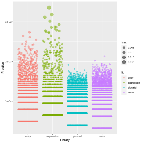
R
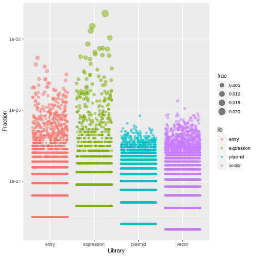
counts %>%
  ggplot(aes(x=lib, y=frac, size=frac, color=lib)) +
  geom_jitter(alpha=0.5, height=0) +
  scale_y_log10() +
  labs(x="Library", y="Fraction")
R
counts <- counts %>%
  arrange(desc(frac)) %>%
  group_by(lib) %>%
  mutate(rank = row_number())

glimpse(counts)
OUTPUT
Rows: 40,000
Columns: 5
Groups: lib [4]
$ peptide <chr> "NKLAPNL", "DNPLDPY", "VEDTTFA", "HSCKITP", "RRRMETN", "DLGQGD…
$ count   <int> 509, 339, 292, 232, 190, 166, 164, 161, 146, 137, 133, 131, 12…
$ lib     <chr> "expression", "expression", "expression", "expression", "expre…
$ frac    <dbl> 0.022756740, 0.015156257, 0.013054947, 0.010372424, 0.00849465…
$ rank    <int> 1, 2, 3, 4, 5, 6, 7, 8, 9, 10, 11, 12, 13, 14, 1, 15, 16, 2, 3…
Challenge
Make a table where there is one row for each peptide, and a column for the rank of the peptide in each library.
That is, there’s one column containing the counts for the plasmid library, one column for the counts in the vector library, and so on.
In this table, assign a unique ID (using row_number()) to each peptide, ranking by count in the expression library. That is, the peptide ranked 1 in the expression library should have ID 1, the peptide ranked 2 in the expression library should have ID 2, and so on.
Assign this new table to a variable ranked.
R
ranked <- counts %>%
  select(lib, peptide, rank) %>%
  pivot_wider(id_cols = "peptide", names_from="lib", values_from = "rank") %>%
  arrange(expression) %>%
  mutate(id = row_number())

ranked
OUTPUT
# A tibble: 10,000 × 6
   peptide expression entry vector plasmid    id
   <chr>        <int> <int>  <int>   <int> <int>
 1 NKLAPNL          1    35    902    1807     1
 2 DNPLDPY          2    80    171     396     2
 3 VEDTTFA          3    92    189     301     3
 4 HSCKITP          4   141    434     757     4
 5 RRRMETN          5   186    541     909     5
 6 DLGQGDE          6   226    766    2197     6
 7 DLCLKKT          7   219    780    1930     7
 8 PHGMDPM          8     4    131     266     8
 9 CGHLPGF          9   288   1097    2934     9
10 HDIIKQH         10   275   1224    2754    10
# … with 9,990 more rows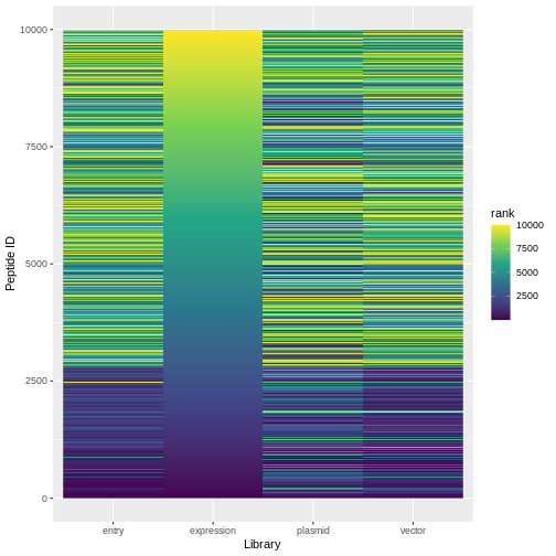
R
ranked %>%
  pivot_longer(expression:plasmid, names_to="lib", values_to="rank") %>%
  ggplot(aes(x=lib, y=id, fill=rank)) +
  geom_raster() +
  scale_fill_viridis_c()+
  labs(x="Library", y="Peptide ID")

Challenge
Create a new table (called expr_enrich) in which you calculate the ‘enrichment score’ of each peptide in the expression library relative to the vector library (that is, \(\frac{\text{fraction in expression library}}{\text{fraction in vector library}}\)). Add a column called rank which ranks the peptides based on this enrichment score
R
expr_enrich <- counts %>%
  filter(lib %in% c("expression", "vector")) %>%
  select(peptide, lib, frac) %>%
  pivot_wider(names_from = lib, values_from = frac) %>%
  mutate(enrichment = expression / vector) %>%
  arrange(desc(enrichment)) %>%
  mutate(rank = row_number())


expr_enrich
OUTPUT
# A tibble: 10,000 × 5
   peptide expression   vector enrichment  rank
   <chr>        <dbl>    <dbl>      <dbl> <int>
 1 NKLAPNL    0.0228  0.000231       98.4     1
 2 DNPLDPY    0.0152  0.000442       34.3     2
 3 CGHLPGF    0.00653 0.000210       31.0     3
 4 HSCKITP    0.0104  0.000336       30.8     4
 5 VEDTTFA    0.0131  0.000442       29.6     5
 6 DLGQGDE    0.00742 0.000252       29.4     6
 7 HDIIKQH    0.00613 0.000210       29.1     7
 8 DLCLKKT    0.00733 0.000252       29.1     8
 9 RRRMETN    0.00849 0.000294       28.9     9
10 PGTAPIT    0.00300 0.000105       28.5    10
# … with 9,990 more rowsR
vec_enrich <- counts %>%
  filter(lib %in% c("plasmid", "vector")) %>%
  select(peptide, lib, frac) %>%
  pivot_wider(names_from = lib, values_from = frac) %>%
  mutate(enrichment = vector / plasmid) %>%
  arrange(desc(enrichment)) %>%
  mutate(rank = row_number())

poor_packagers <- vec_enrich %>%
  filter(enrichment < 1)

poor_packagers
OUTPUT
# A tibble: 5,668 × 5
   peptide    vector   plasmid enrichment  rank
   <chr>       <dbl>     <dbl>      <dbl> <int>
 1 MLCGFYC 0.0000421 0.0000503      0.837  4333
 2 VGCWDVE 0.0000421 0.0000503      0.837  4334
 3 KWVRLEQ 0.0000421 0.0000503      0.837  4335
 4 YMRPDEV 0.0000421 0.0000503      0.837  4336
 5 SFCASIY 0.0000421 0.0000503      0.837  4337
 6 CPLGTGF 0.0000421 0.0000503      0.837  4338
 7 PYNDHMH 0.0000421 0.0000503      0.837  4339
 8 NFNNSQI 0.0000421 0.0000503      0.837  4340
 9 ERVRIFK 0.0000421 0.0000503      0.837  4341
10 RFWAGYK 0.0000421 0.0000503      0.837  4342
# … with 5,658 more rowsR
good_peptides <- expr_enrich %>%
  filter(!peptide %in% poor_packagers$peptide) %>%
  slice_max(order_by=enrichment, n=500)

good_peptides
OUTPUT
# A tibble: 541 × 5
   peptide expression   vector enrichment  rank
   <chr>        <dbl>    <dbl>      <dbl> <int>
 1 NKLAPNL    0.0228  0.000231       98.4     1
 2 DNPLDPY    0.0152  0.000442       34.3     2
 3 CGHLPGF    0.00653 0.000210       31.0     3
 4 HSCKITP    0.0104  0.000336       30.8     4
 5 VEDTTFA    0.0131  0.000442       29.6     5
 6 DLGQGDE    0.00742 0.000252       29.4     6
 7 HDIIKQH    0.00613 0.000210       29.1     7
 8 DLCLKKT    0.00733 0.000252       29.1     8
 9 RRRMETN    0.00849 0.000294       28.9     9
10 PGTAPIT    0.00300 0.000105       28.5    10
# … with 531 more rows
R
write_tsv(good_peptides, file=here::here("good_peptides.tsv"))