Tidy data
Last updated on 2023-01-24 | Edit this page
Estimated time 22 minutes
Overview
Questions
- What is tidy data?
- How can we pivot data frames to make them tidy?
Objectives
- Understand the principles of tidy data
- Use
pivot_longer()andpivot_wider()to create longer or wider data frames
Check Challenge 1 for the solution!
Tidy data
When recording observations, we don’t often give that much thought to how we record the data. Usually we enter data into an excel spreadsheet and care most about entering the data in the easiest way. However, this often results in ‘messy’ data that requires a little bit of massaging before analysis.
There are many possible ways to structure a dataset. For example, if we conducted an experiment where we made two sequencing libraries, in which we have counted the instances of six different barcodes, we could structure the data like this:
OUTPUT
# A tibble: 2 × 7
  library    b1    b2    b3    b4    b5    b6
  <chr>   <int> <int> <int> <int> <int> <int>
1 lib1      384   796   109   404   106   812
2 lib2      102   437   391   782   101   789
In this table, the counts for each barcode are stored in a separate column. The ‘library’ column tells us which library the counts on each row are from.
Conversely, we could keep the counts for each library in a separate column, and the rows can tell us which barcode is being counted:
OUTPUT
# A tibble: 6 × 3
  barcode  lib1  lib2
  <chr>   <int> <int>
1 b1        384   102
2 b2        796   437
3 b3        109   391
4 b4        404   782
5 b5        106   101
6 b6        812   789
We could even structure the table like this:
OUTPUT
# A tibble: 2 × 13
  library `384` `796` `109` `404` `106` `812` `102` `437` `391` `782` `101`
  <chr>   <chr> <chr> <chr> <chr> <chr> <chr> <chr> <chr> <chr> <chr> <chr>
1 lib1    b1    b2    b3    b4    b5    b6    <NA>  <NA>  <NA>  <NA>  <NA>
2 lib2    <NA>  <NA>  <NA>  <NA>  <NA>  <NA>  b1    b2    b3    b4    b5
# … with 1 more variable: `789` <chr>
This is one of the least intuitive ways to structure the data - the columns are the counts (except for the library column), and the rows tell us which barcode had which count.
These are all examples of messy ways to structure the data. There are usually very many ways to make the data messy, but only one ‘Tidy’ format. Being tidy means a dataset has:
- Each variable forms a column.
- Each observation forms a row.
- Each type of observational unit forms a table.
Here, variables record all the values that measure the same attribute (for example library, sample, count), and an observation contains all the measurements on a single unit (like a sequencing run, or a single experiment). Each observational unit (like independent experiments with different variables) should get its own table. This just means that if we ran another experiment with different variables, it should go in a different table.
In our this case, the tidy version looks like this:
R
table1
OUTPUT
# A tibble: 12 × 3
   library barcode count
   <chr>   <chr>   <int>
 1 lib1    b1        384
 2 lib1    b2        796
 3 lib1    b3        109
 4 lib1    b4        404
 5 lib1    b5        106
 6 lib1    b6        812
 7 lib2    b1        102
 8 lib2    b2        437
 9 lib2    b3        391
10 lib2    b4        782
11 lib2    b5        101
12 lib2    b6        789
This is tidy because each column represents a variable (library, barcode and count), each row is an observation (count for a given library and barcode), and we have all the data from this experiment in the one table.
Discussion
Open the excel file readr/untidy_data.xlsx. Do you think this dataset is in a tidy format? Why/why not?
List ways that it could be improved.
Issues with this dataset:
- Doesn’t start in cell A1
- Column names don’t describe contents - information is missing. What do the numbers represent? Better column name would be ‘count’ or similar
- Used a mixture of words and numbers in a column
To make it tidy:
- Columns should be ‘batch’ and ‘count’ (or whatever is being measured)
- Start at cell A1
- How to deal with missing values? As a separate table?
- Or we could have batch 1 and batch 2 as two separate tables
tidyr for tidying data
So if tidy data is the goal, how do we get there? One way is to go back and edit the original file manually. But this is problematic for several reasons:
- You should treat your original data as read-only, and never change it
- Manual edits are not reproducible
- Manual edits can be time-consuming
Instead, we can use tools from the tidyr and dplyr packages for tidying and manipulating tables of data.
Pivoting
The variants on the tables that we saw above are all generated by pivoting the tidy (or ‘long’) version to untidy (in this case, ‘wide’) versions. For example, looking at table1b:
R
table1b
OUTPUT
# A tibble: 6 × 3
  barcode  lib1  lib2
  <chr>   <int> <int>
1 b1        384   102
2 b2        796   437
3 b3        109   391
4 b4        404   782
5 b5        106   101
6 b6        812   789
Another way to think about tidiness is if the names of the column can reflect the data contained in them. It’s a bit misleading to call the columns lib1 and lib2, they actually store counts (and not some other property of the library, such as the barcodes it contains).
We can see that if we were to restructure the lib1 and lib2 columns into two different columns, one that tell us from which library the count came, and one that contains the count value, the dataset would be tidy.
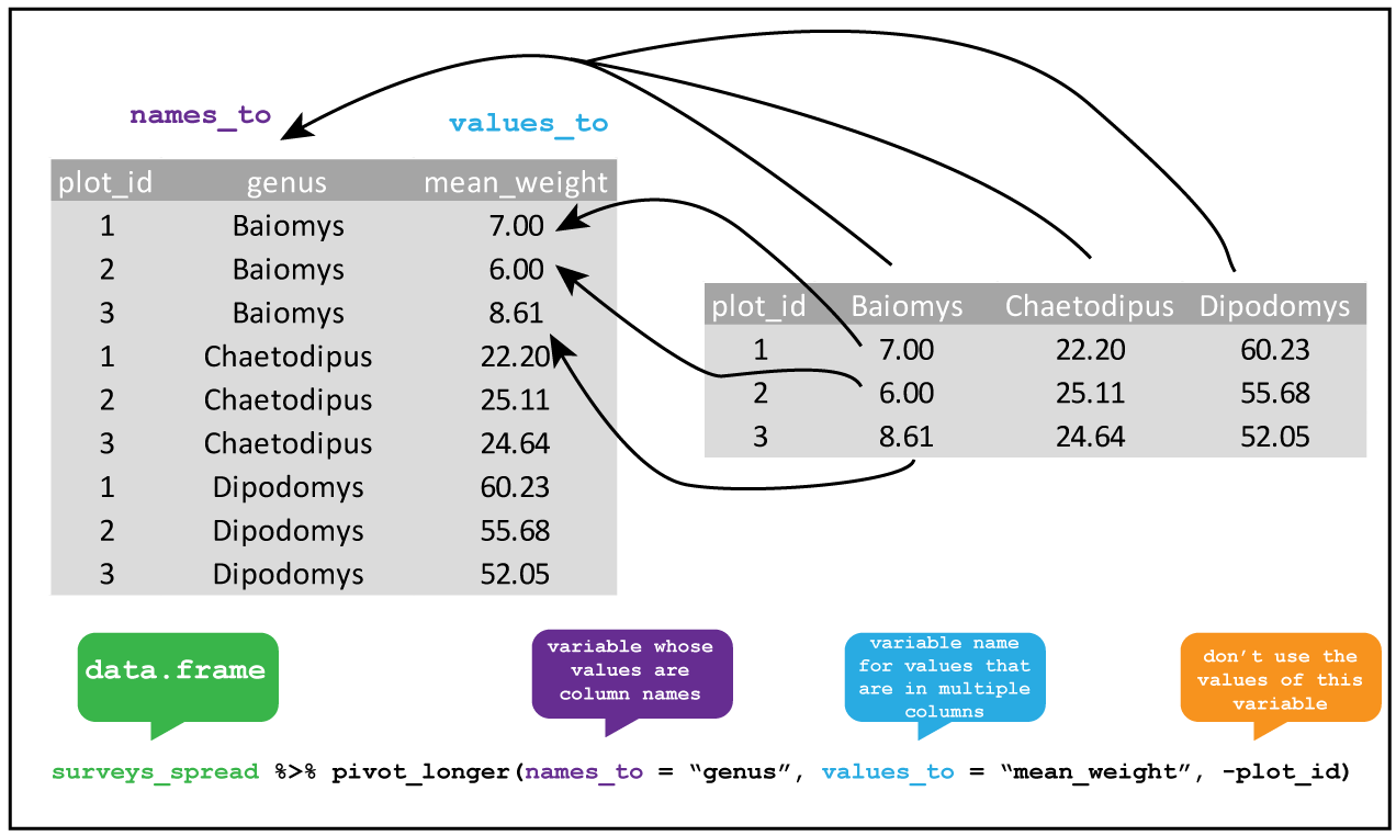
Consolidating columns with pivot_longer()
Knowing this, we can tidy the dataset up using pivot_longer().
R
library(tidyverse)

table1b %>%
  pivot_longer(lib1:lib2, names_to="library", values_to="count")
OUTPUT
# A tibble: 12 × 3
   barcode library count
   <chr>   <chr>   <int>
 1 b1      lib1      384
 2 b1      lib2      102
 3 b2      lib1      796
 4 b2      lib2      437
 5 b3      lib1      109
 6 b3      lib2      391
 7 b4      lib1      404
 8 b4      lib2      782
 9 b5      lib1      106
10 b5      lib2      101
11 b6      lib1      812
12 b6      lib2      789
We can tell that this data is tidy because the column names accurately reflect the data they contain: the count column stores counts, the library column tells us which library the counts came from, and the barcode column tells us which barcode we’re measuring.
Data pipelines with pipes (%>%)
In the code block above, we saw a strange collection of symbols (%>%) after the variable that contained our data. What does it do?
This construct is called the pipe, and comes from the magrittr package (which is part of the tidyverse). You can either type out the three characters seperatly, or use the shortcut Ctrl + Shift + m to insert a pipe.
Let’s consider an example. Say that we have a vector called counts that represents the counts for several vectors in a selection experiment, and we wanted to identify the unique counts, take their log, and then take the mean.
One way to do this is to call each function sequentially, assigning each to an intermediate variable:
R
# generate binomial data to play with
counts <- rbinom(10000, 50, 0.5)

unique_counts <- unique(counts)
log_counts <- log(unique_counts, 10)
mean_log_counts <- mean(log_counts)
This is a bit inefficient because we’ve had to type out the same variable name twice. I often find that when I do things this way, when I change one of the steps but forget to change both the variable names, and end up with weird bugs.
An alternative is to nest all the function calls inside each other:
R
mean_log_counts <- mean(log(unique(counts), 10))
Hopefully you can see why this isn’t a good idea - nested function calls can get very messy, very quickly, especially if the functions have multiple arguments (like log()).
A third way is using the pipe %>% operator, which feeds the output of each function into the next:
R
mean_log_counts <- counts %>%
  unique() %>%
  log(10) %>%
  mean()
This version of the code is cleaner, and the top-to-bottom flow makes the order the functions are applied in more obvious. This way of doing things is very popular, and you’ll see it a lot (for example, in code sample on stack overflow).
There are a few complications to using the pipe which you can read more about here. One that’s worth being aware of is that using lots of pipes can result in long pipelines, and if something goes wrong somewhere in the middle it can be hard to track down exactly where the issue is. In this case, you can use a few intermediate variables to try to figure out which step is going wrong.
Creating more columns with pivot_wider()
We can also do the reverse operation using pivot_wider() (this was how I generated the untidy versions of the tables). But haven’t we just been saying that we should always aspire to keep our data tidy? So why would we ever want to do this?
When working with data in R, the long format does tend to be the most useful, because this is the format that most functions expect data to be in. However, if you want to display the data for a person (rather than for a function in code), the wide format can sometimes be useful for making comparisons. For example, we can easily compare the counts for each barcode in the two libraries in table1b, but the comparison is easy for a person to make when the table is in a long form.
R
table1
OUTPUT
# A tibble: 12 × 3
   library barcode count
   <chr>   <chr>   <int>
 1 lib1    b1        384
 2 lib1    b2        796
 3 lib1    b3        109
 4 lib1    b4        404
 5 lib1    b5        106
 6 lib1    b6        812
 7 lib2    b1        102
 8 lib2    b2        437
 9 lib2    b3        391
10 lib2    b4        782
11 lib2    b5        101
12 lib2    b6        789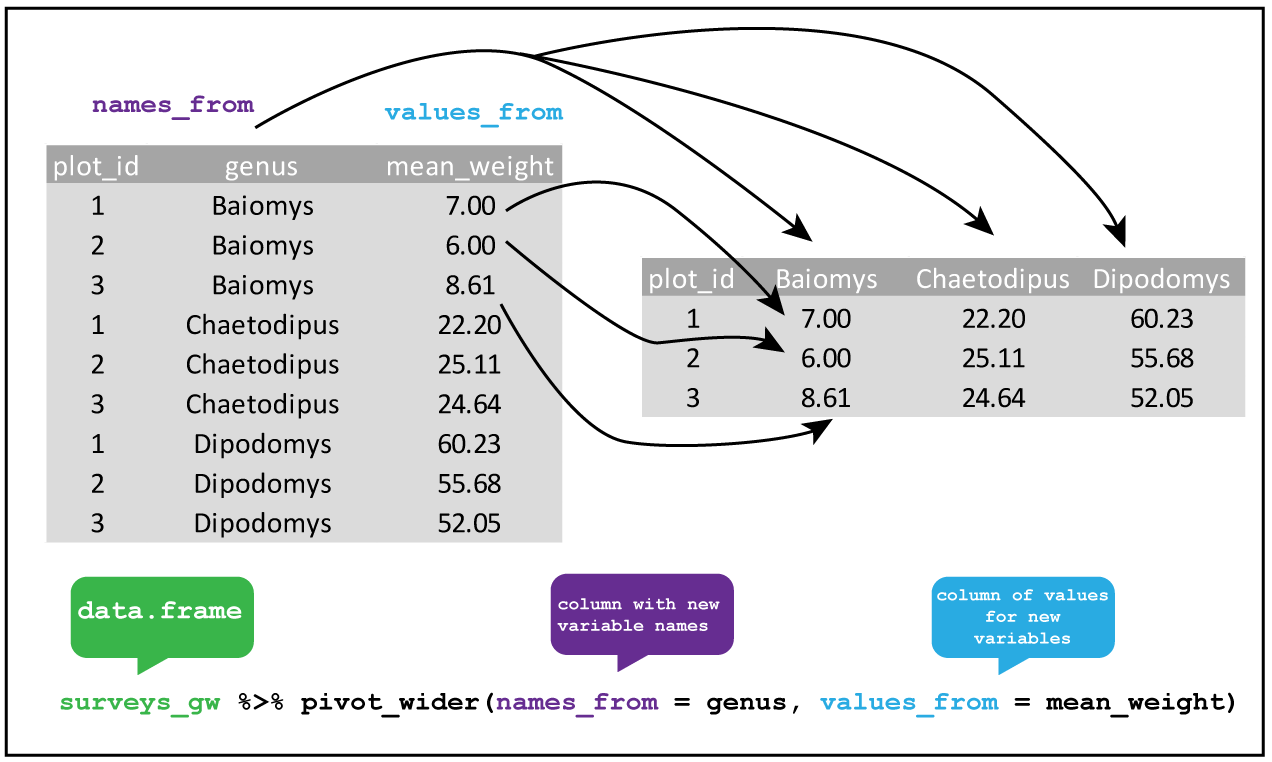
We can pivot our long table to a wide one using pivot_longer().
R
table1 %>%
  pivot_wider(names_from = "library", values_from = "count")
OUTPUT
# A tibble: 6 × 3
  barcode  lib1  lib2
  <chr>   <int> <int>
1 b1        384   102
2 b2        796   437
3 b3        109   391
4 b4        404   782
5 b5        106   101
6 b6        812   789
Other tidyr functions
Tidyr also has a number of other useful functions for tidying up datasets, which include: - Combining columns where multiples pieces of information are spread out (unite()), or spreading out columns which contain data that should be in separate column (separate()) - Adding extra rows to create all possible combinations of the values in multiple columns (expand() and complete) - Handling missing values, for example replacing NA values with something else (replace_na()) or dropping rows that contain NA (drop_na()) - Nesting data within list-columns (nest()), and unnesting such columns (unnest())
While useful, I tend to use these less frequently compared to the pivoting functions, so I leave these to you to explore on your own. You can get an overview of these functions on the tidyr cheatsheet, and in the tidyr documentation.
R
fp <- here::here("episodes", "data", "untidy_data.xlsx")
df <- readxl::read_xlsx(fp, col_names = c("batch_1", "batch_2"),
                        col_types = c("numeric", "numeric"))
ERROR
Error: `path` does not exist: '/home/runner/work/cmri_R_workshop/cmri_R_workshop/site/built/episodes/data/untidy_data.xlsx'R
df %>%
  # we don't know what the values represent, so just call the column 'value'
  pivot_longer(contains("batch"), names_to = "batch", values_to = "value") %>%
  # drop rows that have an NA value
  drop_na(value)
ERROR
Error in UseMethod("pivot_longer"): no applicable method for 'pivot_longer' applied to an object of class "function"Resources and acknowledgments
- tidyr cheatsheet
- Tidy data vignette
- Tidy data paper
- I’ve borrowed figures (and inspiration) from the excellent coding togetheR course material