Bioconductor and other bioinformatics packages
Last updated on 2023-01-24 | Edit this page
Estimated time 22 minutes
Overview
Questions
- What is bioconductor?
- What are some bioconductor packages?
Objectives
- Install bioconductor packages with
BiocManager - Be aware of some
Bioconductor packages
- Use
BiocManager::install(). - In the same way as other
Rpackages. All will have avignettedemonstrating how to use the package, and most will have some other guides demonstrating aspects of the package.
Introduction to Bioconductor
We’ll quickly take a look at theBioconductor ecosystem, a collection of R packages for bioinformatics. Usually these solve specific problems (like RNA-seq analysis or plotting genomic data), so they won’t be as applicable to everyone here.
The goal of this lesson is therefore to let you know about some packages from bioconductor that I’ve found useful, but we won’t actually go into any detail about how to use them. All of the Bioconductor packages have vignettes that will show you how to use the core functionality of the package.
Installing packages with BiocManager
While typically you’d use install.packages() to install R packages, Bioconductor has it’s own package manager. The package manager is called BiocManager, and you can install it as you would any other package:
R
# install BiocManager
install.packages("BiocManager")
You can then use this package to install other Bioconductor packages, for example:
R
BiocManager::install("DESeq2")
Bioconductor also has it’s own release schedule, which are designed to work with particular versions of R.
At the time of writing, the current version is 3.16, which works with R version 4.2.0. If you have an older version of R, you will need to use an older version of Bioconductor as well - there’s a list of the older releases on the Bioconductor website. You can tell BiocManager which release to use:
R
BiocManager::install(version="3.16")
This won’t actually install anything, but all future installs will use version 3.16.
Biostrings
A common task (at least for me) is working with biological sequences (e.g. DNA, RNA, amino acid). A useful package for this is Biostrings.
Install this package with the following code
R
BiocManager::install("Biostrings")
Biostrings contains useful variable and functions for working with sequences. For example, you can translate a nucleotide sequence:
R
# load library
library(biostrings)
R
# create DNAString object
my_seq <- DNAString("GTAAGTGTATGC")

# translate to amino acids
translate(my_seq)
OUTPUT
4-letter AAString object
seq: VSVC
Or calculate the frequency of each nucleotide:
R
alphabetFrequency(my_seq)
OUTPUT
A C G T M R W S Y K V H D B N - + .
3 1 4 4 0 0 0 0 0 0 0 0 0 0 0 0 0 0
Or the codon frequencies
R
trinucleotideFrequency(my_seq)
OUTPUT
AAA AAC AAG AAT ACA ACC ACG ACT AGA AGC AGG AGT ATA ATC ATG ATT CAA CAC CAG CAT
  0   0   1   0   0   0   0   0   0   0   0   1   0   0   1   0   0   0   0   0
CCA CCC CCG CCT CGA CGC CGG CGT CTA CTC CTG CTT GAA GAC GAG GAT GCA GCC GCG GCT
  0   0   0   0   0   0   0   0   0   0   0   0   0   0   0   0   0   0   0   0
GGA GGC GGG GGT GTA GTC GTG GTT TAA TAC TAG TAT TCA TCC TCG TCT TGA TGC TGG TGT
  0   0   0   0   2   0   1   0   1   0   0   1   0   0   0   0   0   1   0   1
TTA TTC TTG TTT
  0   0   0   0
It also contains a codon table
R
GENETIC_CODE
OUTPUT
TTT TTC TTA TTG TCT TCC TCA TCG TAT TAC TAA TAG TGT TGC TGA TGG CTT CTC CTA CTG
"F" "F" "L" "L" "S" "S" "S" "S" "Y" "Y" "*" "*" "C" "C" "*" "W" "L" "L" "L" "L"
CCT CCC CCA CCG CAT CAC CAA CAG CGT CGC CGA CGG ATT ATC ATA ATG ACT ACC ACA ACG
"P" "P" "P" "P" "H" "H" "Q" "Q" "R" "R" "R" "R" "I" "I" "I" "M" "T" "T" "T" "T"
AAT AAC AAA AAG AGT AGC AGA AGG GTT GTC GTA GTG GCT GCC GCA GCG GAT GAC GAA GAG
"N" "N" "K" "K" "S" "S" "R" "R" "V" "V" "V" "V" "A" "A" "A" "A" "D" "D" "E" "E"
GGT GGC GGA GGG
"G" "G" "G" "G"
attr(,"alt_init_codons")
[1] "TTG" "CTG"
It has many more features which you can explore if you need to use this package.
Plotting genomic information
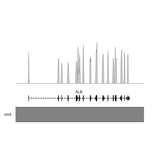
Another relatively common task for me is plotting genomic information. There are a number of ways to do this, but here I’ll just give one example - plotting the density of SNPs in the human albumin gene (ALB).
First, I grabbed the SNP information for this gene from gnomAD as a csv, and read in this information using readr::read_csv()
R
# load data
alb <- readr::read_csv(here::here("episodes", "data", "gnomAD_v3.1.2_ENSG00000163631_2022_11_25_11_56_32.csv"), show_col_types = FALSE)
Next, we need to convert the SNP locations into a GRanges object - this is an object from the GenomicRanges package that is designed to store genomic coordinates and associated metadata. I won’t go into detail about this either, but you can find more information about this package in the documentation.
R
# for pipe
library(magrittr, quietly=TRUE)
OUTPUT
Attaching package: 'magrittr'OUTPUT
The following object is masked from 'package:GenomicRanges':

    subtract
R
alb_gr <- alb %>%
  # add "chr" to chromosome number
  dplyr::mutate(Chromosome = paste0("chr", Chromosome)) %>%
  # convert to GRanges object
  GenomicRanges::makeGRangesFromDataFrame(
    seqnames.field="Chromosome",
    start.field = "Position",
    end.field="Position",
    keep.extra.columns = FALSE
  )

alb_gr
OUTPUT
GRanges object with 850 ranges and 0 metadata columns:
        seqnames    ranges strand
           <Rle> <IRanges>  <Rle>
    [1]     chr4  73397115      *
    [2]     chr4  73397120      *
    [3]     chr4  73397122      *
    [4]     chr4  73397122      *
    [5]     chr4  73397123      *
    ...      ...       ...    ...
  [846]     chr4  73421175      *
  [847]     chr4  73421187      *
  [848]     chr4  73421188      *
  [849]     chr4  73421189      *
  [850]     chr4  73421193      *
  -------
  seqinfo: 1 sequence from an unspecified genome; no seqlengths
Now we have the data loaded, we’re ready to start making the plot.
KaryoploteR
Here I’m more or less following part of the karyploteR tutorial.
This is human data, so we plot the albumin locus in the human genome. I used the UCSC genome brower to identify the coordinates for ALB (roughly chr4:73,394,000-73,425,000), but you could equally use Ensembl.
R
library(karyoploteR)
# this package contains transcript information for the human genome
library(TxDb.Hsapiens.UCSC.hg38.knownGene)
R
# region to plot
region <- "chr4:73,394,000-73,425,000"

# draw axis
kp <- plotKaryotype(zoom = region)

# transcript information
genes.data <- makeGenesDataFromTxDb(TxDb.Hsapiens.UCSC.hg38.knownGene,
                                    karyoplot=kp,
                                    plot.transcripts = TRUE,
                                    plot.transcripts.structure = TRUE)
OUTPUT
  1662 genes were dropped because they have exons located on both strands
  of the same reference sequence or on more than one reference sequence,
  so cannot be represented by a single genomic range.
  Use 'single.strand.genes.only=FALSE' to get all the genes in a
  GRangesList object, or use suppressMessages() to suppress this message.
R
# add gene names
genes.data <- addGeneNames(genes.data)
OUTPUT
Loading required package: org.Hs.eg.dbOUTPUT
R
# merge overlapping transcripts
genes.data <- mergeTranscripts(genes.data)

# draw genes
kpPlotGenes(kp, data=genes.data, r0=0, r1=0.15)
# draw SNP density
kpPlotDensity(kp, data=alb_gr, window=100, r0=0.3, r1=1)
circlize
Another package for plotting genomic information is circlize, which plots chromosome in a circle rather than in a linear format. I won’t cover this in any detail, but you can check out the documentation for more information.
RNA-seq
One common tasks people use Bioconductor packages for is RNA-seq analysis. The steps in RNA-seq analysis are roughly the following:
- Alignment of reads using splice-aware mapper (I use
STAR) - Counting reads aligned to each exon/transcript/gene (I use
htseq-countfromHTSeq) - Downstream analysis with counts - batch correction, differential expression, gene ontology, pathway analysis, etc
While it’s possible to do the entire RNA-seq analysis pipeline, from reads to differential expressed genes, in R, you’ll notice that I usually do the first two steps using other software. This mostly comes down to momentum - this is how I was taught - but also has to do with the perception that R easier to use but slower and more memory-intensive than other languages (like C++, the language in which STAR is written).
We could spend a whole session (or workshop) on RNA-seq, so instead of trying to cover all of this material, I’ll instead link to several resources that might be helpful for experimental design and data processing.
- Notes on RNA-seq experimental design (Very important!! Without proper experimental design you are only wasting time and money.)
- The DESeq2 vignette
- The EdgeR vignette
- Materials from a two-day RNA-seq workshop
- Sample differential gene expression workflow
If you’re more interested in single cell analysis, the workflow is in principle the same, but there is the added complication of counting barcodes from each cell. If your data is from a 10X workflow, the easiest way to go from reads to counts is using their cellranger pipeline. Once you have the count matrices, you can then use R packages for further analysis.
Resources
- BiocManager vignette
- Biostrings lab
- Biostrings documentation
- karyoploteR documentation
- circlize documentation
- Notes on RNA-seq experimental design (Very important!! Without proper experimental design you are only wasting time and money.)
- The DESeq2 vignette
- The EdgeR vignette
- Materials from a two-day RNA-seq workshop
- Sample differential gene expression workflow
- Seurat documentation
- Monocle3 documentation