Using R markdown for notebooks and documents

Estimated time 27 minutes

Overview

Questions

• How do you write a notebook or document using R Markdown?

Objectives

• Explain how to use markdown documents and notebooks
• Demonstrate how to include a header, markdown elements, pieces of code and code outputs
• Discuss how to render documents and notebooks

Do I need to do this lesson?

If you can answer the following questions, you can skip this lesson.

1. What does a R markdown header look like?
2. How do you insert headings in an R markdown file?
3. How do you insert chunks in an R markdown file, and what do they look like?
4. What is the difference between an R markdown document and notebook?
5. How do you render an R markdown file?

Show me the solution

1. It looks something like this

YAML

---
title: "Habits"
author: Jane Doe
date: March 22, 2005
output: html_document
---

2. Use one two four hashes (#) at the start of the line.
3. Insert code blocks by typing them manually, in the menu bar under Code > Insert Chunk, or with the shortcut Cmd/Ctrl + Option + i. They look like this:

MARKDOWN

```{r chunk-name}
y <- 2
print(y)
```

4. For a notebook, an output is generated every time you save it. A document is only rendered when you Knit it.
5. Use the Knit or Preview buttons, or use the function rmarkdown::render(). For notebooks, just save the file to automatically render the file with any outputs that currently appear in Rstudio.

Rmarkdown for reproducible, documented analyis

---

For a long time, most R code was written in scripts. These are just plain old text files, usually with the file extension .R, which contain R code. Any documentation in these scripts was in the form of comments, and any graphic generated had to be saved to file (or viewed in a window, then closed).

This paradigm worked, but it was lacking an integrated view of the results of the analysis. This is the problem that knitr and R markdown were developed to address.

R markdown allows the user to create notebooks and documents that contain text elements (formatted using markdown), and R code. If I’ve ever sent you a .html file containing some results, this is how I generated it. Other formats are possible for data export, including .pdf, but I tend to always use .html for it’s interactive elements.

Documents you create are rendered into the final output format that you’ve specified, by running all the code and combining the outputs it with your markdown text.

Although simple, this approach is powerful; I wrote all the content on this website using R markdown files.

Rmarkdown header

R markdown files always start with a header, which is formatted in YAML, and at it’s most basic looks something like this:

YAML

---
title: "R Notebook"
output: html_notebook
---

That’s it: just a title and an output.

Output types

When you create a .Rmd file, you’ll have to choose if you want it to be a notebook (output: html_notebook), a document (output: html_document), or some other output type (for example, output: pdf_document).

Notebooks and documents are very similar, and the only difference between html documents and notebooks is that a .html file is created with your analysis every time you save a notebook, whereas an output file will only be created for a document when you tell RStudio to render it.

If you want, you can add an author and a date, for example:

YAML

---
title: "Habits"
author: Jane Doe
date: "22 November 2022"
output: html_document
---

Sometimes I want the date to be updated every time I render the document. You can do this by replacing the date with some R code.

YAML

---
title: "Habits"
author: Jane Doe
date: "`r Sys.Date()`"
output: html_document
---

There are also lots of options for html documents and notebooks. I often use:

YAML

---
title: "Habits"
author: Jane Doe
date: "`r Sys.Date()`"
output:
  html_document:
    keep_md: true
    df_print: paged
    toc: true
    toc_float:
      collapsed: false
      smooth_scroll: false
    code_folding: hide
---

You can also add parameters in your header that you can use throughout your code:

YAML

---
title: "Habits"
author: Jane Doe
date: "`r Sys.Date()`"
output:
  html_document:
    keep_md: true
    df_print: paged
    toc: true
    toc_float:
      collapsed: false
      smooth_scroll: false
    code_folding: hide
params:
  test: true
  species: "human"
---

You can then refer to these parameters using the syntax params$test and params$species.

Markdown

Writing the markdown part of the file is are pretty simple. Use # for headings.

MARKDOWN

# Largest heading
## Large heading
### Medium heading
#### Small heading

To create paragraphs, leave at least one blank line between text.

MARKDOWN

This is a paragraph.

This is a different paragraph.

To add a line break (to prevent sentences from running on from one another), add two spaces at the end of the line.

MARKDOWN

This is a line.  
This is another line.

To add emphasis, use * or _.

MARKDOWN

This text is **bold**.
This text is __also bold__.
This text is in *italics*.
This text is also in _italics_.
This text is both ***bold and in italics***.
___Same here___.

To create a block quote, add > to the start of each line.

MARKDOWN

> This will be a quote
>
> that's all in the same block

To make a list, use numbers or dashes.

MARKDOWN

This is an unordered list:

 - element a
 - element b
 - element c
 
This is an ordered list:

1. element 1
2. element 2
3. element 3
 

If you want to display code, use backticks:

MARKDOWN

This is `inline` code.

```r
print("this is an R code block")
```

To add images, use this syntax:

MARKDOWN

![Caption for figure](/path/to/figure.png)

You can add links using parentheses and brackets:

MARKDOWN

You can read more in the [documentation](https://www.markdownguide.org/basic-syntax/)

Adding code

Adding code blocks is also easy. Use the shortcut Cmd/ctrl + Option + i. You can also check what the shortcut is on your machine in the menu bar under Code > Insert Chunk.

Code blocks look like this:

MARKDOWN

```{r chunk-name}
y <- 2
print(y)
```

There are lots of options to control how the code block and it’s output is displayed. For example:

MARKDOWN

```{r chunk-name2, echo=FALSE}
print("this code block won't appear in the output, but its output will")
```

MARKDOWN

```{r chunk-name3, include=FALSE}
print("this code block won't appear in the output, and neither will it's output")
```

If your code block produces a plot, the plot will appear in the report. You can change the size of the plot with options as well.

MARKDOWN

```{r chunk-name4, fig.width=8, fig.height=8}
tibble(
  group = c("A", "A", "B", "B"),
  y = runif(4)
) %>% 
  ggplot(aes(x=group, y = y)) +
  geom_point()
```

You can also apply options to all chunks using knitr::set_opts() at the top of your file.

MD

```r
knitr::opts_chunk$set(
  echo=FALSE, fig.width = 6, fig.height = 6
)
```

Code block names

Code blocks can be named or unnamed. If they have a name, it’ll be the first argument in the curly braces ({}) after the three backticks that enclose the block.

Make sure that you don’t have two code blocks with the same name in your file, otherwise you won’t be able to render it!

Inline code

You can also insert inline code in R markdown by using the syntax r my_expression. However, I don’t tend to do this much in documents because every time I re-open the file, using variables in these code blocks cause problems (because they don’t exist yet).

If you’re going to use inline code a lot, I’d recommend you stick to using R markdown documents instead of notebooks.

Running code blocks

Run individual lines of code in a chunk by pressing Ctrl + Enter, or run the whole chunk using Ctrl + Shift + Enter (or the ‘play’ symbol at the top right). You can also highlight particular pieces of a line that you want to run, and use Ctrl + Enter to run them.

Rendering notebooks

---

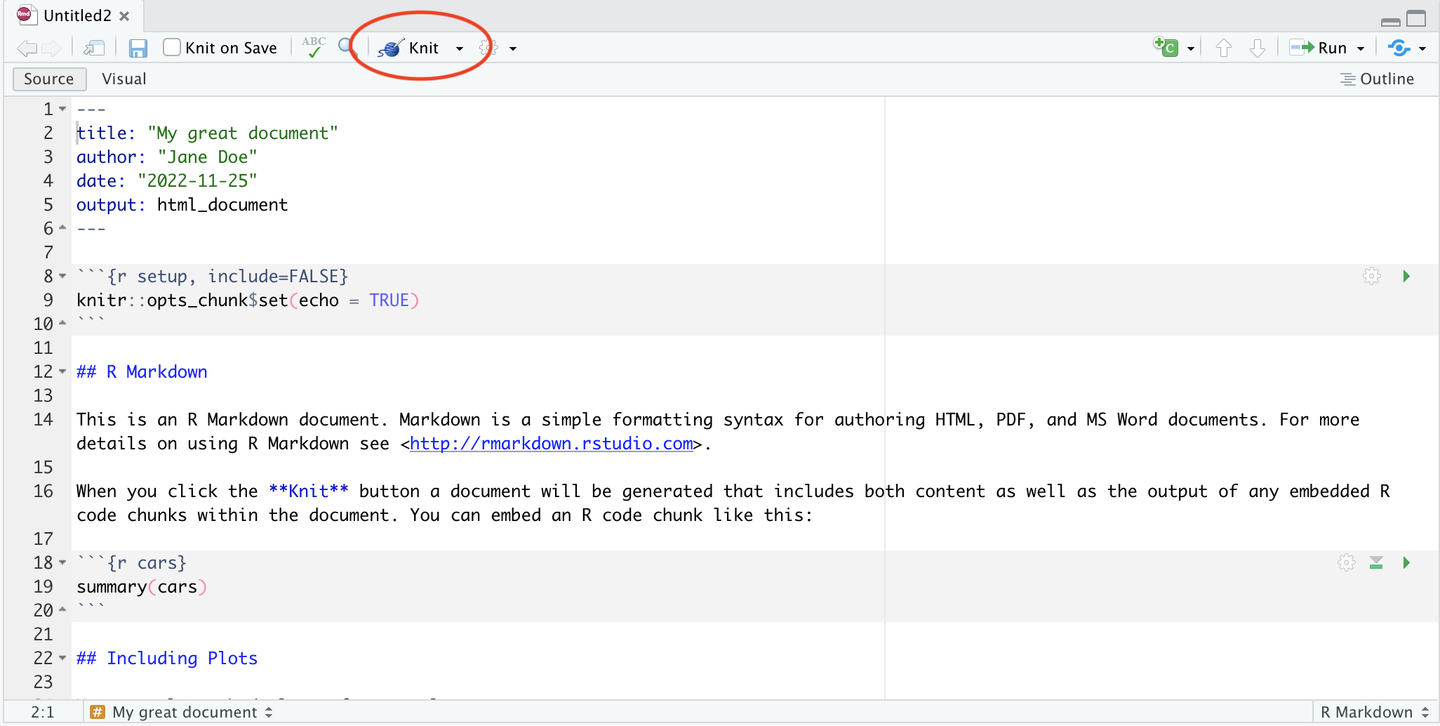
There are a few different ways you can render your R markdown file. The easiest is to use the dedicated button in Rstudio. For documents, it’ at the top of your document and looks like this:

Button for knitting documents

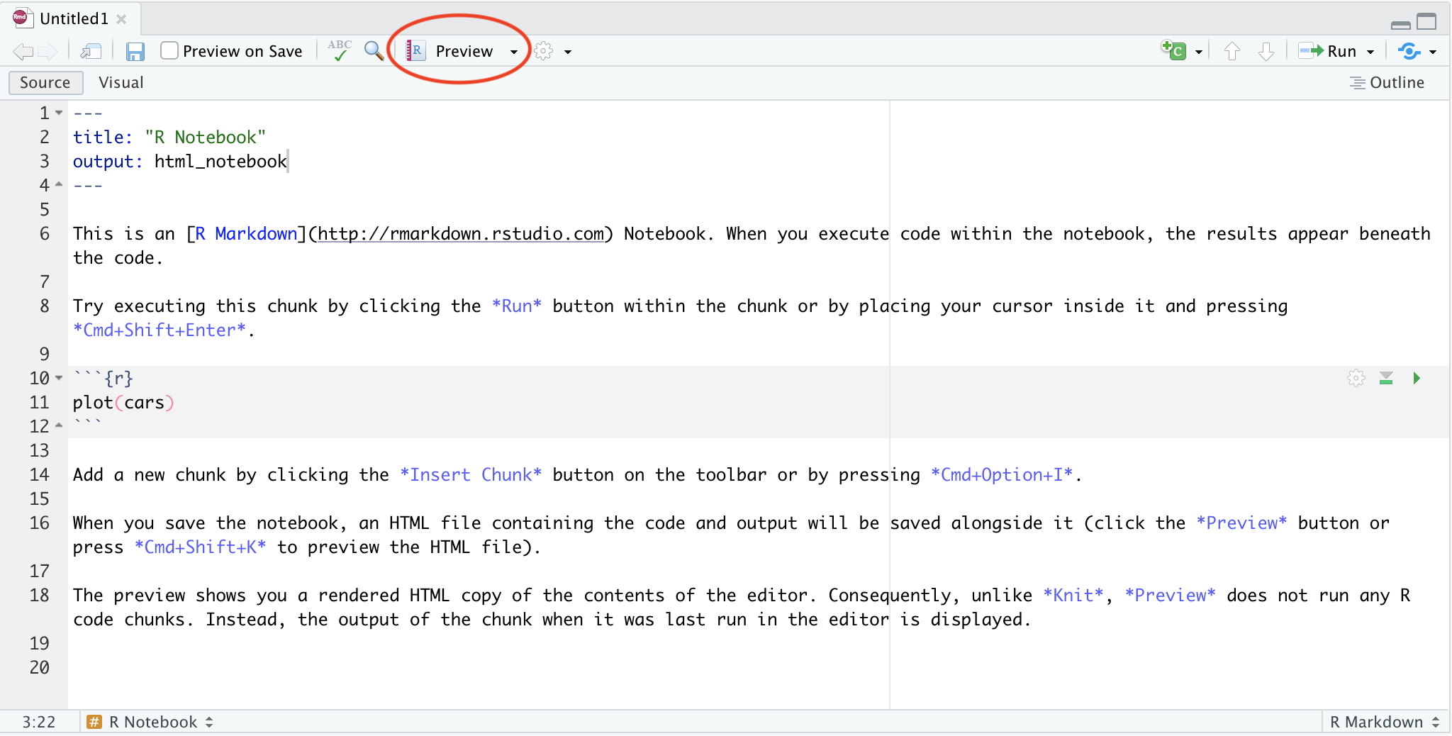
For notebooks, you don’t need to manually render - every time you save the file, R will knit it for you. But if you want to see what the notebook will look like, you can press the preview button:

Button for knitting noteooks

You can also render your notebook using code:

R

rmarkdown::render("/path/to/file.Rmd")

If you set parameters, you can change them when you render the notebook:

R

rmarkdown::render("/path/to/file.Rmd", params = list(test=FALSE, speces="macaque"))

Other file types

---

There are also a number of other outputs you can produce from your R markdown other than html notebooks and documents. In particular, I’ve been playing around with slides using Quatro and ioslides. They can be a little tricky compared to power point, and a bit slow to render if your analysis is compute-heavy, but I think they’re worth considering!

This area is actively being developed, so it’s worth trying out new technologies when they are available.

References

---

• R markdown cheetsheet
• R markdown guide
• R markdown cookbook
• Markdown guide

Keypoints

• Specify document-wide properties in the header
• Use markdown element to format text
• Use code chunks to run R code
• Render your notebook using the buttons in Rstudio, or using rmarkdown::render()