Data wrangling
Last updated on 2023-01-24 | Edit this page
Overview
Questions
- What are the main
dplyrverbs? - How can I analyse data within groups?
Objectives
- Know how to use the main
dplyrverbs - Use
group_by()to aggregate and manipulate within groups
Do I need to do this lesson?
If you already have experience with dplyr, you can skip this lesson if you can answer all the following questions.
- Load in the weather data from the
readrandreadxl‘do I need to do this lesson’ challenge. In the process, create a column calledfilethat contains the filename for each row. - Create a column called
citywith the name of the city (‘brisbane’, or ‘sydney’). - What is the median minimum (
min_temp_c) and maximum (max_temp_c) temperature in the observations for each city? - Count the number of days when there were more than 10 hours of sunshine (
sunshine_hours) in each city. - A cold cloudy day is one where there were fewer than 10 hours of sunshine, and the maximum temperature was less than 15 degrees. A hot sunny day is one where there were more than 10 hours of sunshine, and the maximum temperature was more than than 25 degrees. Calculate the the mean relative humidity at 9am (
rel_humid_9am_pc) and 3pm (rel_humid_3pm_pc) on days that were hot and sunny, cold and cloudy, or neither. - What is the mean maximum temperature on the 5 hottest days in each city?
- Add a column ranking the days by minimum temperature for each city, where the coldest day for each is rank 1, the next coldest is rank 2, etc.
- Generate a forecast for each city using the code below. If a cloudy day is one where there are 10 or fewer hours of sunshine, on how many days was the forecast accurate?
R
library(lubridate)
OUTPUT
Loading required package: timechangeOUTPUT
Attaching package: 'lubridate'OUTPUT
The following objects are masked from 'package:base':

    date, intersect, setdiff, union
R
# generate days
days <- seq(ymd('2022-11-01'),ymd('2022-11-29'), by = '1 day')

# forecast is the same in each city - imagine it's a country-wide forecast
forecast <- tibble(
  date = rep(days)
) %>%
  # toss a coin
  mutate(forecast = sample(c("cloudy", "sunny"), size = n(), replace=TRUE))
ERROR
Error in tibble(date = rep(days)) %>% mutate(forecast = sample(c("cloudy", : could not find function "%>%"R
# 1. Load in the weather data from the `readr` and `readxl` 'do I need to do this lesson' challenge

library(tidyverse)
OUTPUT
── Attaching packages ─────────────────────────────────────── tidyverse 1.3.2 ──
✔ ggplot2 3.4.0      ✔ purrr   1.0.1
✔ tibble  3.1.8      ✔ dplyr   1.0.10
✔ tidyr   1.2.1      ✔ stringr 1.4.1
✔ readr   2.1.3      ✔ forcats 0.5.2
── Conflicts ────────────────────────────────────────── tidyverse_conflicts() ──
✖ lubridate::as.difftime() masks base::as.difftime()
✖ lubridate::date()        masks base::date()
✖ dplyr::filter()          masks stats::filter()
✖ lubridate::intersect()   masks base::intersect()
✖ dplyr::lag()             masks stats::lag()
✖ lubridate::setdiff()     masks base::setdiff()
✖ lubridate::union()       masks base::union()
R
wthr_path <- here::here("episodes", "data", c("weather_brisbane.csv", "weather_sydney.csv"))

# column types
col_types <- list(
  date = col_date(format="%Y-%m-%d"),
  min_temp_c = col_double(),
  max_temp_c = col_double(),
  rainfall_mm = col_double(),
  evaporation_mm = col_double(),
  sunshine_hours = col_double(),
  dir_max_wind_gust = col_character(),
  speed_max_wind_gust_kph = col_double(),
  time_max_wind_gust = col_time(),
  temp_9am_c = col_double(),
  rel_humid_9am_pc = col_integer(),
  cloud_amount_9am_oktas = col_double(),
  wind_direction_9am = col_character(),
  wind_speed_9am_kph = col_double(),
  MSL_pressure_9am_hPa = col_double(),
  temp_3pm_c = col_double(),
  rel_humid_3pm_pc = col_double(),
  cloud_amount_3pm_oktas = col_double(),
  wind_direction_3pm = col_character(),
  wind_speed_3pm_kph = col_double(),
  MSL_pressure_3pm_hPa = col_double()
)

# read in data
weather <- read_csv(wthr_path, skip=10,
                    col_types=col_types, col_names = names(col_types),
                    id = "file"
                    )
ERROR
Error: '/home/runner/work/cmri_R_workshop/cmri_R_workshop/site/built/episodes/data/weather_brisbane.csv' does not exist.R
glimpse(weather)
ERROR
Error in glimpse(weather): object 'weather' not foundNothing much new here if you already did the readr episode.
R
# 2. Create a column with the name of the city ('brisbane', or 'sydney').

weather <- weather %>%
  mutate(city = stringr::str_extract(file, "brisbane|sydney"))
ERROR
Error in mutate(., city = stringr::str_extract(file, "brisbane|sydney")): object 'weather' not foundR
# 3. What is the median minimum (`min_temp_c`) and maximum (`max_temp_c`)
# temperature in the observations for each city?

weather %>%
  group_by(city) %>%
  summarise(median_min_temp = median(min_temp_c),
            median_max_temp = median(max_temp_c, na.rm=TRUE))
ERROR
Error in group_by(., city): object 'weather' not foundWe need na.rm=TRUE for the maximum column because this column contains NA values
R
#4. Count the number of days when there were more than 10 hours of sunshine
# (`sunshine_hours`) in each city.

weather %>%
  mutate(sunny = sunshine_hours > 10) %>%
  count(sunny, city)
ERROR
Error in mutate(., sunny = sunshine_hours > 10): object 'weather' not foundHere I did count() as a shortcut for group_by() and summarise(), but the long way works too.
R
#5. A cold cloudy day is one where there were fewer than 10 hours of sunshine,
# and the maximum temperature was less than 15 degrees.
# A hot sunny day is one where there were more than 10 hours of sunshine,
# and the maximum temperature was more than than 25 degrees.
# Calculate the the mean relative humidity at 9am (`rel_humid_9am_pc`) and
# 3pm (`rel_humid_3pm_pc`) on days that were hot and sunny, cold and cloudy, or neither.

weather %>%
  mutate(day = case_when(
    sunshine_hours > 10 & max_temp_c > 25 ~ "hot_sunny",
    sunshine_hours <= 10 & max_temp_c < 15 ~ "cold_cloudy",
    TRUE ~ "neither"
  )) %>%
  group_by(day) %>%
  summarise(mean_humid_9am = mean(rel_humid_9am_pc),
            mean_humid_3pm = mean(rel_humid_3pm_pc, na.rm=TRUE))
ERROR
Error in mutate(., day = case_when(sunshine_hours > 10 & max_temp_c > : object 'weather' not foundThere were no cold cloudy days in this dataset.
R
# 6. What is the mean maximum temperature on the 5 hottest days in each city?
weather %>%
  group_by(city) %>%
  slice_max(order_by = max_temp_c, n = 5, with_ties=FALSE) %>%
  summarise(mean_max_temp = mean(max_temp_c, na.rm=TRUE))
ERROR
Error in group_by(., city): object 'weather' not foundHere I use slice_max(), but there are more complicated ways to solve this using other dplyr verbs.
R
#7. Add a column ranking the days by minimum temperature for each city,
# where the coldest day for each is rank 1, the next coldest is rank 2, etc.

weather %>%
  group_by(city) %>%
  arrange(min_temp_c) %>%
  mutate(rank = row_number())
ERROR
Error in group_by(., city): object 'weather' not foundI tend to use the combination of arrange(), mutate() and row_number() for adding ranks, but there are probably other ways of achieving the same end.
R
# 8.  If a cloudy day is one where there are 10 or fewer hours of sunshine,
# on how many days was the forecast accurate?

weather %>%
  left_join(forecast, by="date") %>%
  mutate(cloudy_or_sunny = ifelse(sunshine_hours > 10, "sunny", "cloudy")) %>%
  mutate(forecast_accurate = forecast == cloudy_or_sunny) %>%
  count(forecast_accurate)
ERROR
Error in left_join(., forecast, by = "date"): object 'weather' not foundSee challenge 7 for an alternative way of solving this problem.
Manipulating data with dplyr
So once we have our data in a tidy format, what do we do with it? For analysis, I often turn to the dplyr package, which contains several useful functions for manipulating tables of data.
To illustrate the functions of this package, we’ll use a dataset of weather observations in Brisbane and Sydney from the Bureau of Meterology.
These files are called weather_brisbane.csv and weather_sydney.csv.
First, we load both files using readr:
R
# load tidyverse
library(tidyverse)

# data files
# data files - readr can also read data from the internet
data_dir <- "https://raw.githubusercontent.com/szsctt/cmri_R_workshop/main/episodes/data/"
data_files <- file.path(data_dir, c("weather_sydney.csv", "weather_brisbane.csv"))


# column types
col_types <- list(
  date = col_date(format="%Y-%m-%d"),
  min_temp_c = col_double(),
  max_temp_c = col_double(),
  rainfall_mm = col_double(),
  evaporation_mm = col_double(),
  sunshine_hours = col_double(),
  dir_max_wind_gust = col_character(),
  speed_max_wind_gust_kph = col_double(),
  time_max_wind_gust = col_time(),
  temp_9am_c = col_double(),
  rel_humid_9am_pc = col_integer(),
  cloud_amount_9am_oktas = col_double(),
  wind_direction_9am = col_character(),
  wind_speed_9am_kph = col_double(),
  MSL_pressure_9am_hPa = col_double(),
  temp_3pm_c = col_double(),
  rel_humid_3pm_pc = col_double(),
  cloud_amount_3pm_oktas = col_double(),
  wind_direction_3pm = col_character(),
  wind_speed_3pm_kph = col_double(),
  MSL_pressure_3pm_hPa = col_double()
)

# read in data
weather <- readr::read_csv(data_files, skip=10,
                           col_types=col_types, col_names = names(col_types),
                           id="file")
Creating summaries with summarise()
First, we would like to know what the mean minimum and maximum temperatures were overall. For this, we can use summarise():
R
weather %>%
  summarise(mean_min_temp = mean(min_temp_c),
            mean_max_temp = mean(max_temp_c))
OUTPUT
# A tibble: 1 × 2
  mean_min_temp mean_max_temp
          <dbl>         <dbl>
1          16.0            NA
Notice that the mean_max_temp is NA, because we had some NA values in this column. In R we use NA for missing values. So how does one take the mean of some numbers, some of which are missing? We can’t so the answer is also a missing value. We can, however, tell the mean() function to ignore the missing values using na.rm=TRUE:
R
weather %>%
  summarise(mean_min_temp = mean(min_temp_c),
            mean_max_temp = mean(max_temp_c, na.rm=TRUE))
OUTPUT
# A tibble: 1 × 2
  mean_min_temp mean_max_temp
          <dbl>         <dbl>
1 16.0 26.2R
weather %>%
  summarise(median_min_temp = median(min_temp_c),
            median_max_temp = median(max_temp_c, na.rm=TRUE))
OUTPUT
# A tibble: 1 × 2
  median_min_temp median_max_temp
            <dbl>           <dbl>
1            15.9            25.3
dplyr also has some special functions that are designed to be used inside of other functions. For example, if we want to know how many observations there were of the minimum and maximum temperatures, we could use n(). Or if we wanted to know how many different directions the maximum wind gust had, we can use n_distinct().
R
weather %>%
  summarise(n_days_observed = n(),
            n_wind_dir = n_distinct(dir_max_wind_gust))
OUTPUT
# A tibble: 1 × 2
  n_days_observed n_wind_dir
            <int>      <int>
1              57         15
Grouped summaries with group_by()
However, all of these summaries have combined the observations for Sydney and Brisbane. It probably makes sense to group the observations by city, and then compute the summary statistics. For this, we can use group_by().
If you use group_by() on a tibble, it doesn’t actually look like it changes that much.
R
weather %>%
  group_by(file)
OUTPUT
# A tibble: 57 × 22
# Groups: file [2]
file date min_t…¹ max_t…² rainf…³ evapo…⁴ sunsh…⁵ dir_m…⁶ speed…⁷
<chr> <date> <dbl> <dbl> <dbl> <dbl> <dbl> <chr> <dbl>
1 https://r… 2022-11-01 18.2 24 0.2 4.6 9.5 WNW 69
2 https://r… 2022-11-02 11.1 20.5 0.6 13 12.8 W 67
3 https://r… 2022-11-03 11.1 22 0 7.8 8.9 W 56
4 https://r… 2022-11-04 13.4 23.1 1 6 5.7 SSE 26
5 https://r… 2022-11-05 13.4 23.6 0.2 4.4 11.8 ENE 37
6 https://r… 2022-11-06 13.3 24 0 4 12.1 ENE 39
7 https://r… 2022-11-07 15.4 24.2 0 9.8 12.3 NE 41
8 https://r… 2022-11-08 16 24.2 1.2 8 11 ENE 35
9 https://r… 2022-11-09 14.9 24.2 0.2 8 10.3 E 33
10 https://r… 2022-11-10 14.9 24.4 0 7.8 9.3 ENE 43
# … with 47 more rows, 13 more variables: time_max_wind_gust <time>,
# temp_9am_c <dbl>, rel_humid_9am_pc <int>, cloud_amount_9am_oktas <dbl>,
# wind_direction_9am <chr>, wind_speed_9am_kph <dbl>,
# MSL_pressure_9am_hPa <dbl>, temp_3pm_c <dbl>, rel_humid_3pm_pc <dbl>,
# cloud_amount_3pm_oktas <dbl>, wind_direction_3pm <chr>,
# wind_speed_3pm_kph <dbl>, MSL_pressure_3pm_hPa <dbl>, and abbreviated
# variable names ¹min_temp_c, ²max_temp_c, ³rainfall_mm, ⁴evaporation_mm, …The only difference is that when you print it out, it tells you that it’s grouped by file. However, a grouped data frame interacts differently with other dplyr verbs, such as summary.
R
weather %>%
  group_by(file) %>%
  summarise(median_min_temp = median(min_temp_c),
            median_max_temp = median(max_temp_c, na.rm=TRUE))
OUTPUT
# A tibble: 2 × 3
file media…¹ media…²
<chr> <dbl> <dbl>
1 https://raw.githubusercontent.com/szsctt/cmri_R_workshop/main… 16.7 27.7
2 https://raw.githubusercontent.com/szsctt/cmri_R_workshop/main… 15.4 24.2
# … with abbreviated variable names ¹median_min_temp, ²median_max_tempNow we get the median temperature for both Sydney and Brisbane.
R
weather %>%
  group_by(file, dir_max_wind_gust) %>%
  summarise(max_max_wind_gust = max(speed_max_wind_gust_kph))
OUTPUT
`summarise()` has grouped output by 'file'. You can override using the
`.groups` argument.
OUTPUT
# A tibble: 24 × 3
# Groups: file [2]
file dir_m…¹ max_m…²
<chr> <chr> <dbl>
1 https://raw.githubusercontent.com/szsctt/cmri_R_workshop/mai… E 35
2 https://raw.githubusercontent.com/szsctt/cmri_R_workshop/mai… ENE 37
3 https://raw.githubusercontent.com/szsctt/cmri_R_workshop/mai… ESE 35
4 https://raw.githubusercontent.com/szsctt/cmri_R_workshop/mai… NE 26
5 https://raw.githubusercontent.com/szsctt/cmri_R_workshop/mai… NNE 35
6 https://raw.githubusercontent.com/szsctt/cmri_R_workshop/mai… NW 48
7 https://raw.githubusercontent.com/szsctt/cmri_R_workshop/mai… S 39
8 https://raw.githubusercontent.com/szsctt/cmri_R_workshop/mai… W 44
9 https://raw.githubusercontent.com/szsctt/cmri_R_workshop/mai… WNW 33
10 https://raw.githubusercontent.com/szsctt/cmri_R_workshop/mai… WSW 43
# … with 14 more rows, and abbreviated variable names ¹dir_max_wind_gust,
# ²max_max_wind_gustR
weather %>%
  group_by(file, dir_max_wind_gust) %>%
  summarise(max_max_wind_gust = max(speed_max_wind_gust_kph)) %>%
  ungroup() %>%
  pivot_wider(id_cols=file, names_from = "dir_max_wind_gust", values_from = "max_max_wind_gust")
OUTPUT
`summarise()` has grouped output by 'file'. You can override using the
`.groups` argument.
OUTPUT
# A tibble: 2 × 16
  file       E   ENE   ESE    NE   NNE    NW     S     W   WNW   WSW  `NA`   NNW
  <chr>  <dbl> <dbl> <dbl> <dbl> <dbl> <dbl> <dbl> <dbl> <dbl> <dbl> <dbl> <dbl>
1 https…    35    37    35    26    35    48    39    44    33    43    NA    NA
2 https…    33    50    26    41    NA    NA    54    83    69    54    NA    46
# … with 3 more variables: SSE <dbl>, SSW <dbl>, SW <dbl>
Do you prefer the long or wide form of the table?
Creating new columns with mutate()
It’s kind of annoying that we have the whole file names, rather than just the names of the cities. To fix this, we can create (or overwrite) columns with mutate().

dplyr::mutate() image creditFor example, the stringr::str_extract() function extracts a matching pattern from a string:
R
stringr::str_extract(data_files, "sydney|brisbane")
OUTPUT
[1] "sydney" "brisbane"Regular expressions for pattern matching in strings
The second argument to str_extract() is a regular expression, or regex. Using regular expressions is a hugely flexible way to specify a pattern to match in a string, but it’s a somewhat complicated topic that I won’t go into here. If you’re interested in learning more, you can look at the stringr documentation on regular expressions.
We can use mutate() to apply the str_extract() function to the file column
R
weather <- weather %>%
  mutate(city = stringr::str_extract(file, "sydney|brisbane"))
weather
OUTPUT
# A tibble: 57 × 23
file date min_t…¹ max_t…² rainf…³ evapo…⁴ sunsh…⁵ dir_m…⁶ speed…⁷
<chr> <date> <dbl> <dbl> <dbl> <dbl> <dbl> <chr> <dbl>
1 https://r… 2022-11-01 18.2 24 0.2 4.6 9.5 WNW 69
2 https://r… 2022-11-02 11.1 20.5 0.6 13 12.8 W 67
3 https://r… 2022-11-03 11.1 22 0 7.8 8.9 W 56
4 https://r… 2022-11-04 13.4 23.1 1 6 5.7 SSE 26
5 https://r… 2022-11-05 13.4 23.6 0.2 4.4 11.8 ENE 37
6 https://r… 2022-11-06 13.3 24 0 4 12.1 ENE 39
7 https://r… 2022-11-07 15.4 24.2 0 9.8 12.3 NE 41
8 https://r… 2022-11-08 16 24.2 1.2 8 11 ENE 35
9 https://r… 2022-11-09 14.9 24.2 0.2 8 10.3 E 33
10 https://r… 2022-11-10 14.9 24.4 0 7.8 9.3 ENE 43
# … with 47 more rows, 14 more variables: time_max_wind_gust <time>,
# temp_9am_c <dbl>, rel_humid_9am_pc <int>, cloud_amount_9am_oktas <dbl>,
# wind_direction_9am <chr>, wind_speed_9am_kph <dbl>,
# MSL_pressure_9am_hPa <dbl>, temp_3pm_c <dbl>, rel_humid_3pm_pc <dbl>,
# cloud_amount_3pm_oktas <dbl>, wind_direction_3pm <chr>,
# wind_speed_3pm_kph <dbl>, MSL_pressure_3pm_hPa <dbl>, city <chr>, and
# abbreviated variable names ¹min_temp_c, ²max_temp_c, ³rainfall_mm, …Now if we repeat the same summary as before, we get an output that’s a bit easier to read.
R
weather %>%
  group_by(city) %>%
  summarise(median_min_temp = median(min_temp_c),
            median_max_temp = median(max_temp_c, na.rm=TRUE))
OUTPUT
# A tibble: 2 × 3
  city     median_min_temp median_max_temp
  <chr>              <dbl>           <dbl>
1 brisbane            16.7            27.7
2 sydney              15.4            24.2
Mutating multiple columns with across()
Let’s imagine that the calibration was wrong for both temperature sensors, and all the temperature measurements are out by 1°C. We’d like to add 1 to each of the temperature measurements. There are multiple columns that contain temperatures, so we could do this:
R
weather %>%
  mutate(min_temp_c = min_temp_c + 1,
         max_temp_c = max_temp_c + 1,
         temp_9am_c = temp_9am_c + 1,
         temp_3pm_c = temp_3pm_c + 1)
OUTPUT
# A tibble: 57 × 23
file date min_t…¹ max_t…² rainf…³ evapo…⁴ sunsh…⁵ dir_m…⁶ speed…⁷
<chr> <date> <dbl> <dbl> <dbl> <dbl> <dbl> <chr> <dbl>
1 https://r… 2022-11-01 19.2 25 0.2 4.6 9.5 WNW 69
2 https://r… 2022-11-02 12.1 21.5 0.6 13 12.8 W 67
3 https://r… 2022-11-03 12.1 23 0 7.8 8.9 W 56
4 https://r… 2022-11-04 14.4 24.1 1 6 5.7 SSE 26
5 https://r… 2022-11-05 14.4 24.6 0.2 4.4 11.8 ENE 37
6 https://r… 2022-11-06 14.3 25 0 4 12.1 ENE 39
7 https://r… 2022-11-07 16.4 25.2 0 9.8 12.3 NE 41
8 https://r… 2022-11-08 17 25.2 1.2 8 11 ENE 35
9 https://r… 2022-11-09 15.9 25.2 0.2 8 10.3 E 33
10 https://r… 2022-11-10 15.9 25.4 0 7.8 9.3 ENE 43
# … with 47 more rows, 14 more variables: time_max_wind_gust <time>,
# temp_9am_c <dbl>, rel_humid_9am_pc <int>, cloud_amount_9am_oktas <dbl>,
# wind_direction_9am <chr>, wind_speed_9am_kph <dbl>,
# MSL_pressure_9am_hPa <dbl>, temp_3pm_c <dbl>, rel_humid_3pm_pc <dbl>,
# cloud_amount_3pm_oktas <dbl>, wind_direction_3pm <chr>,
# wind_speed_3pm_kph <dbl>, MSL_pressure_3pm_hPa <dbl>, city <chr>, and
# abbreviated variable names ¹min_temp_c, ²max_temp_c, ³rainfall_mm, …But it’s a bit annoying to type out each column. Instead, we can use across() inside mutate() to apply the same transformation to all columns whose name contains the string “temp”. The syntax is a little complicated, so don’t worry if you don’t get it straight away. We use the contains() function to get the columns we want (by matching the regex “temp”), and then to each of these columns we add one - the . will be replaced by the name of each column when the expression is evaluated.
R
weather %>%
  mutate(across(contains("temp"), ~.+1))
OUTPUT
# A tibble: 57 × 23
file date min_t…¹ max_t…² rainf…³ evapo…⁴ sunsh…⁵ dir_m…⁶ speed…⁷
<chr> <date> <dbl> <dbl> <dbl> <dbl> <dbl> <chr> <dbl>
1 https://r… 2022-11-01 19.2 25 0.2 4.6 9.5 WNW 69
2 https://r… 2022-11-02 12.1 21.5 0.6 13 12.8 W 67
3 https://r… 2022-11-03 12.1 23 0 7.8 8.9 W 56
4 https://r… 2022-11-04 14.4 24.1 1 6 5.7 SSE 26
5 https://r… 2022-11-05 14.4 24.6 0.2 4.4 11.8 ENE 37
6 https://r… 2022-11-06 14.3 25 0 4 12.1 ENE 39
7 https://r… 2022-11-07 16.4 25.2 0 9.8 12.3 NE 41
8 https://r… 2022-11-08 17 25.2 1.2 8 11 ENE 35
9 https://r… 2022-11-09 15.9 25.2 0.2 8 10.3 E 33
10 https://r… 2022-11-10 15.9 25.4 0 7.8 9.3 ENE 43
# … with 47 more rows, 14 more variables: time_max_wind_gust <time>,
# temp_9am_c <dbl>, rel_humid_9am_pc <int>, cloud_amount_9am_oktas <dbl>,
# wind_direction_9am <chr>, wind_speed_9am_kph <dbl>,
# MSL_pressure_9am_hPa <dbl>, temp_3pm_c <dbl>, rel_humid_3pm_pc <dbl>,
# cloud_amount_3pm_oktas <dbl>, wind_direction_3pm <chr>,
# wind_speed_3pm_kph <dbl>, MSL_pressure_3pm_hPa <dbl>, city <chr>, and
# abbreviated variable names ¹min_temp_c, ²max_temp_c, ³rainfall_mm, …Equivalently, we could also use a function to make the transformation.
R
weather %>%
  mutate(across(contains("temp"), function(x){
    return(x+1)
  }))
OUTPUT
# A tibble: 57 × 23
file date min_t…¹ max_t…² rainf…³ evapo…⁴ sunsh…⁵ dir_m…⁶ speed…⁷
<chr> <date> <dbl> <dbl> <dbl> <dbl> <dbl> <chr> <dbl>
1 https://r… 2022-11-01 19.2 25 0.2 4.6 9.5 WNW 69
2 https://r… 2022-11-02 12.1 21.5 0.6 13 12.8 W 67
3 https://r… 2022-11-03 12.1 23 0 7.8 8.9 W 56
4 https://r… 2022-11-04 14.4 24.1 1 6 5.7 SSE 26
5 https://r… 2022-11-05 14.4 24.6 0.2 4.4 11.8 ENE 37
6 https://r… 2022-11-06 14.3 25 0 4 12.1 ENE 39
7 https://r… 2022-11-07 16.4 25.2 0 9.8 12.3 NE 41
8 https://r… 2022-11-08 17 25.2 1.2 8 11 ENE 35
9 https://r… 2022-11-09 15.9 25.2 0.2 8 10.3 E 33
10 https://r… 2022-11-10 15.9 25.4 0 7.8 9.3 ENE 43
# … with 47 more rows, 14 more variables: time_max_wind_gust <time>,
# temp_9am_c <dbl>, rel_humid_9am_pc <int>, cloud_amount_9am_oktas <dbl>,
# wind_direction_9am <chr>, wind_speed_9am_kph <dbl>,
# MSL_pressure_9am_hPa <dbl>, temp_3pm_c <dbl>, rel_humid_3pm_pc <dbl>,
# cloud_amount_3pm_oktas <dbl>, wind_direction_3pm <chr>,
# wind_speed_3pm_kph <dbl>, MSL_pressure_3pm_hPa <dbl>, city <chr>, and
# abbreviated variable names ¹min_temp_c, ²max_temp_c, ³rainfall_mm, …Filtering rows with filter()
Let’s say that now we want information about days that were cloudy - for example, those where there were fewer than 10 sunshine hours. We can use filter() to get only those rows.

dplyr::filter() image creditR
weather %>%
  filter(sunshine_hours < 10)
OUTPUT
# A tibble: 19 × 23
file date min_t…¹ max_t…² rainf…³ evapo…⁴ sunsh…⁵ dir_m…⁶ speed…⁷
<chr> <date> <dbl> <dbl> <dbl> <dbl> <dbl> <chr> <dbl>
1 https://r… 2022-11-01 18.2 24 0.2 4.6 9.5 WNW 69
2 https://r… 2022-11-03 11.1 22 0 7.8 8.9 W 56
3 https://r… 2022-11-04 13.4 23.1 1 6 5.7 SSE 26
4 https://r… 2022-11-10 14.9 24.4 0 7.8 9.3 ENE 43
5 https://r… 2022-11-11 14.9 24.9 0 7.8 9.1 ENE 39
6 https://r… 2022-11-12 16 27.9 0 7.8 9.5 ESE 26
7 https://r… 2022-11-13 18.9 25.6 0 6.4 1.7 NNW 46
8 https://r… 2022-11-15 16.2 24.9 0.2 9.6 9.2 SW 33
9 https://r… 2022-11-16 13 21.6 0.8 8 9.1 S 54
10 https://r… 2022-11-27 17 26.8 0 8 3.7 WSW 54
11 https://r… 2022-11-28 17.1 23.8 8.8 3.8 8.9 SSW 31
12 https://r… 2022-11-08 14.7 25.2 0 10 9.9 ESE 33
13 https://r… 2022-11-14 20.6 28.8 0 9.8 8.4 ENE 26
14 https://r… 2022-11-20 20.8 34.5 0 8.8 5.7 NW 48
15 https://r… 2022-11-22 20.6 30.7 0 11.6 9.2 ENE 28
16 https://r… 2022-11-23 18.4 27.6 0 8.8 4.4 WNW 22
17 https://r… 2022-11-24 16.9 28.6 0 8 2.7 NE 20
18 https://r… 2022-11-27 19.8 29.4 0 8.8 6.1 NW 24
19 https://r… 2022-11-28 21.1 31 21.4 5.4 6.1 S 39
# … with 14 more variables: time_max_wind_gust <time>, temp_9am_c <dbl>,
# rel_humid_9am_pc <int>, cloud_amount_9am_oktas <dbl>,
# wind_direction_9am <chr>, wind_speed_9am_kph <dbl>,
# MSL_pressure_9am_hPa <dbl>, temp_3pm_c <dbl>, rel_humid_3pm_pc <dbl>,
# cloud_amount_3pm_oktas <dbl>, wind_direction_3pm <chr>,
# wind_speed_3pm_kph <dbl>, MSL_pressure_3pm_hPa <dbl>, city <chr>, and
# abbreviated variable names ¹min_temp_c, ²max_temp_c, ³rainfall_mm, …R
weather %>%
  filter(sunshine_hours > 10) %>%
  group_by(city) %>%
  summarise(n_days = n())
OUTPUT
# A tibble: 2 × 2
  city     n_days
  <chr>     <int>
1 brisbane     19
2 sydney       17
There were more days with more than 10 hours of sunlight in Brisbane than in Sydney. I’ll let you draw your own conclusions.
Complex filters with case_when()
Let’s say we wanted to keep only the rows from sunny, warm days and cloudy, cold days. We could do this just with one logical expression.
R
weather %>%
  filter((sunshine_hours > 10 & max_temp_c > 25) | (sunshine_hours < 10 & max_temp_c < 15))
OUTPUT
# A tibble: 19 × 23
file date min_t…¹ max_t…² rainf…³ evapo…⁴ sunsh…⁵ dir_m…⁶ speed…⁷
<chr> <date> <dbl> <dbl> <dbl> <dbl> <dbl> <chr> <dbl>
1 https://r… 2022-11-14 18.1 27.9 37.6 4.2 10.8 W 67
2 https://r… 2022-11-20 18 27.4 0.8 7.8 13.3 W 70
3 https://r… 2022-11-23 13.7 28.3 0 8 12.4 W 54
4 https://r… 2022-11-24 15.8 25.4 0 11.2 12 E 33
5 https://r… 2022-11-05 15.5 25.1 0 8.6 12.2 E 30
6 https://r… 2022-11-06 15.6 25.6 0 8.2 12.7 E 31
7 https://r… 2022-11-07 15.5 25.7 0 7.4 12.6 ENE 37
8 https://r… 2022-11-09 14.7 25.3 0 8.4 12.4 ESE 30
9 https://r… 2022-11-10 15.9 25.7 0 8.6 12.5 E 35
10 https://r… 2022-11-11 14.4 26.2 0 9.4 12.1 E 22
11 https://r… 2022-11-12 15.8 28.4 0 7.4 10.5 NE 26
12 https://r… 2022-11-13 17.6 27.7 0 7.2 12.4 NNE 33
13 https://r… 2022-11-15 20 33.3 0 5.6 12.9 WNW 30
14 https://r… 2022-11-16 16.6 30.1 0 8.2 12.5 WSW 43
15 https://r… 2022-11-18 13.7 27 0 7.4 12.7 ENE 24
16 https://r… 2022-11-19 15.1 28.3 0 8 12.5 NNE 35
17 https://r… 2022-11-21 21.2 34.3 6.6 10.4 10.9 WNW 33
18 https://r… 2022-11-25 17.6 32.4 0 4.2 12.5 NE 26
19 https://r… 2022-11-26 17.3 33.9 0 9.6 12.8 E 35
# … with 14 more variables: time_max_wind_gust <time>, temp_9am_c <dbl>,
# rel_humid_9am_pc <int>, cloud_amount_9am_oktas <dbl>,
# wind_direction_9am <chr>, wind_speed_9am_kph <dbl>,
# MSL_pressure_9am_hPa <dbl>, temp_3pm_c <dbl>, rel_humid_3pm_pc <dbl>,
# cloud_amount_3pm_oktas <dbl>, wind_direction_3pm <chr>,
# wind_speed_3pm_kph <dbl>, MSL_pressure_3pm_hPa <dbl>, city <chr>, and
# abbreviated variable names ¹min_temp_c, ²max_temp_c, ³rainfall_mm, …But you can imagine that with more conditions, this can get a bit messy. I prefer to use case_when() in such situations:
R
weather %>%
  filter(case_when(
    sunshine_hours > 10 & max_temp_c > 25 ~ TRUE,
    sunshine_hours < 10 & max_temp_c < 15 ~ TRUE,
    TRUE ~ FALSE
  ))
OUTPUT
# A tibble: 19 × 23
file date min_t…¹ max_t…² rainf…³ evapo…⁴ sunsh…⁵ dir_m…⁶ speed…⁷
<chr> <date> <dbl> <dbl> <dbl> <dbl> <dbl> <chr> <dbl>
1 https://r… 2022-11-14 18.1 27.9 37.6 4.2 10.8 W 67
2 https://r… 2022-11-20 18 27.4 0.8 7.8 13.3 W 70
3 https://r… 2022-11-23 13.7 28.3 0 8 12.4 W 54
4 https://r… 2022-11-24 15.8 25.4 0 11.2 12 E 33
5 https://r… 2022-11-05 15.5 25.1 0 8.6 12.2 E 30
6 https://r… 2022-11-06 15.6 25.6 0 8.2 12.7 E 31
7 https://r… 2022-11-07 15.5 25.7 0 7.4 12.6 ENE 37
8 https://r… 2022-11-09 14.7 25.3 0 8.4 12.4 ESE 30
9 https://r… 2022-11-10 15.9 25.7 0 8.6 12.5 E 35
10 https://r… 2022-11-11 14.4 26.2 0 9.4 12.1 E 22
11 https://r… 2022-11-12 15.8 28.4 0 7.4 10.5 NE 26
12 https://r… 2022-11-13 17.6 27.7 0 7.2 12.4 NNE 33
13 https://r… 2022-11-15 20 33.3 0 5.6 12.9 WNW 30
14 https://r… 2022-11-16 16.6 30.1 0 8.2 12.5 WSW 43
15 https://r… 2022-11-18 13.7 27 0 7.4 12.7 ENE 24
16 https://r… 2022-11-19 15.1 28.3 0 8 12.5 NNE 35
17 https://r… 2022-11-21 21.2 34.3 6.6 10.4 10.9 WNW 33
18 https://r… 2022-11-25 17.6 32.4 0 4.2 12.5 NE 26
19 https://r… 2022-11-26 17.3 33.9 0 9.6 12.8 E 35
# … with 14 more variables: time_max_wind_gust <time>, temp_9am_c <dbl>,
# rel_humid_9am_pc <int>, cloud_amount_9am_oktas <dbl>,
# wind_direction_9am <chr>, wind_speed_9am_kph <dbl>,
# MSL_pressure_9am_hPa <dbl>, temp_3pm_c <dbl>, rel_humid_3pm_pc <dbl>,
# cloud_amount_3pm_oktas <dbl>, wind_direction_3pm <chr>,
# wind_speed_3pm_kph <dbl>, MSL_pressure_3pm_hPa <dbl>, city <chr>, and
# abbreviated variable names ¹min_temp_c, ²max_temp_c, ³rainfall_mm, …Essentially, case_when() looks at each condition in turn, and if the left part of the expression (before the ~) evaluates to TRUE, then it returns whatever is on the right of the ~.
- We first ask if this row has more than ten sunshine hours and a maximum temperature of more than 25 - if this is the case, we return
TRUE(andfilter()retains this row). - Next, we ask if the row has less than ten sunshine hours and a maximum temperature of less than 15, in which case we also return
TRUE. - If both these statements are
FALSE, then theTRUEon the next line ensures that we don’t keep those rows by always returningFALSE.
Challenge 4: Using case_when() with mutate()
case_when() is also quite useful in combination with mutate().
For example, let’s suppose you want to compare the mean relative humidity on about cloudy cold days and sunny hot days.
You can first use mutate() and case_when() to create a column that tells which of these categories the day belongs to (hot_sunny, cold_cloudy, or neither), and then use group_by() and summarise() to get the mean relative humidity at 9am and 3pm.
Write the code to compute this.
R
weather %>%
  mutate(day_type = case_when(
    sunshine_hours > 10 & max_temp_c > 25 ~ "hot_sunny",
    sunshine_hours < 10 & max_temp_c < 15 ~ "cold_cloudy",
    TRUE ~ "neither"
  )) %>%
  group_by(day_type) %>%
  summarise(mean_rel_humid_9am = mean(rel_humid_9am_pc, na.rm=TRUE),
            mean_rel_humid_3pm = mean(rel_humid_3pm_pc, na.rm=TRUE))
OUTPUT
# A tibble: 2 × 3
  day_type  mean_rel_humid_9am mean_rel_humid_3pm
  <chr>                  <dbl>              <dbl>
1 hot_sunny               48.3               41.2
2 neither                 58.3               49.5
Notice that we didn’t actually have any cold cloudy days, but hot sunny days seem to be less humid.
Filter within groups with slice_xxx()
There are three slice functions that you can use to filter your data: slice_min(), slice_max() and slice_sample(). I usually use them together with group_by() to filter within groups.
use slice_max()
R
weather %>%
  group_by(city) %>%
  slice_max(order_by=max_temp_c, n=1)
OUTPUT
# A tibble: 2 × 23
# Groups: city [2]
file date min_t…¹ max_t…² rainf…³ evapo…⁴ sunsh…⁵ dir_m…⁶ speed…⁷
<chr> <date> <dbl> <dbl> <dbl> <dbl> <dbl> <chr> <dbl>
1 https://ra… 2022-11-20 20.8 34.5 0 8.8 5.7 NW 48
2 https://ra… 2022-11-23 13.7 28.3 0 8 12.4 W 54
# … with 14 more variables: time_max_wind_gust <time>, temp_9am_c <dbl>,
# rel_humid_9am_pc <int>, cloud_amount_9am_oktas <dbl>,
# wind_direction_9am <chr>, wind_speed_9am_kph <dbl>,
# MSL_pressure_9am_hPa <dbl>, temp_3pm_c <dbl>, rel_humid_3pm_pc <dbl>,
# cloud_amount_3pm_oktas <dbl>, wind_direction_3pm <chr>,
# wind_speed_3pm_kph <dbl>, MSL_pressure_3pm_hPa <dbl>, city <chr>, and
# abbreviated variable names ¹min_temp_c, ²max_temp_c, ³rainfall_mm, …If you want the minimum values instead, use slice_min() and if you want a random sample, use slice_sample().
R
weather %>%
  group_by(city) %>%
  # use with_ties to ensure we only get five rows
  slice_max(order_by=max_temp_c, n=5, with_ties = FALSE) %>%
  summarise(
    mean_temp = mean(max_temp_c)
  )
OUTPUT
# A tibble: 2 × 2
  city     mean_temp
  <chr>        <dbl>
1 brisbane      33.7
2 sydney        27.7
Ooof, Brisbane was hot! Maybe this changes your conclusion about which city is better.
Selecting columns with select()
If you want to drop or only retain columns from your table, use select().

dplyr::select() image creditFor example, we added a city column to our table, so we can drop the file column that also contains this information.
R
weather %>%
  select(-file)
OUTPUT
# A tibble: 57 × 22
date min_temp_c max_t…¹ rainf…² evapo…³ sunsh…⁴ dir_m…⁵ speed…⁶ time_…⁷
<date> <dbl> <dbl> <dbl> <dbl> <dbl> <chr> <dbl> <time>
1 2022-11-01 18.2 24 0.2 4.6 9.5 WNW 69 06:50
2 2022-11-02 11.1 20.5 0.6 13 12.8 W 67 12:54
3 2022-11-03 11.1 22 0 7.8 8.9 W 56 07:41
4 2022-11-04 13.4 23.1 1 6 5.7 SSE 26 23:24
5 2022-11-05 13.4 23.6 0.2 4.4 11.8 ENE 37 15:20
6 2022-11-06 13.3 24 0 4 12.1 ENE 39 16:12
7 2022-11-07 15.4 24.2 0 9.8 12.3 NE 41 11:44
8 2022-11-08 16 24.2 1.2 8 11 ENE 35 15:55
9 2022-11-09 14.9 24.2 0.2 8 10.3 E 33 12:37
10 2022-11-10 14.9 24.4 0 7.8 9.3 ENE 43 17:10
# … with 47 more rows, 13 more variables: temp_9am_c <dbl>,
# rel_humid_9am_pc <int>, cloud_amount_9am_oktas <dbl>,
# wind_direction_9am <chr>, wind_speed_9am_kph <dbl>,
# MSL_pressure_9am_hPa <dbl>, temp_3pm_c <dbl>, rel_humid_3pm_pc <dbl>,
# cloud_amount_3pm_oktas <dbl>, wind_direction_3pm <chr>,
# wind_speed_3pm_kph <dbl>, MSL_pressure_3pm_hPa <dbl>, city <chr>, and
# abbreviated variable names ¹max_temp_c, ²rainfall_mm, ³evaporation_mm, …Alternatively, if we only wanted to keep the date, city and the 3pm observations, we can do this as well.
R
weather %>%
  select(date, city, contains("3pm"))
OUTPUT
# A tibble: 57 × 8
date city temp_3pm_c rel_humid_3pm_pc cloud…¹ wind_…² wind_…³ MSL_p…⁴
<date> <chr> <dbl> <dbl> <dbl> <chr> <dbl> <dbl>
1 2022-11-01 sydney 23.1 30 2 WNW 31 992
2 2022-11-02 sydney 19.7 29 1 SW 22 1006.
3 2022-11-03 sydney 20 42 7 SE 20 1017.
4 2022-11-04 sydney 22.8 55 5 ENE 17 1027.
5 2022-11-05 sydney 22.2 60 2 ENE 24 1027.
6 2022-11-06 sydney 23.1 59 1 E 26 1023.
7 2022-11-07 sydney 23.4 58 2 ENE 24 1021.
8 2022-11-08 sydney 24 59 2 ENE 24 1020.
9 2022-11-09 sydney 23.6 46 1 ENE 26 1022.
10 2022-11-10 sydney 24.1 55 1 ENE 24 1019.
# … with 47 more rows, and abbreviated variable names ¹cloud_amount_3pm_oktas,
# ²wind_direction_3pm, ³wind_speed_3pm_kph, ⁴MSL_pressure_3pm_hPaSorting rows with arrange()
You can re-order the rows in a table by the values in one or more columns using arrange().
 Here I sort for the hottest days, using
 desc() to get the maximum temperatures in descending order.R
weather %>%
  arrange(desc(max_temp_c))
OUTPUT
# A tibble: 57 × 23
file date min_t…¹ max_t…² rainf…³ evapo…⁴ sunsh…⁵ dir_m…⁶ speed…⁷
<chr> <date> <dbl> <dbl> <dbl> <dbl> <dbl> <chr> <dbl>
1 https://r… 2022-11-20 20.8 34.5 0 8.8 5.7 NW 48
2 https://r… 2022-11-21 21.2 34.3 6.6 10.4 10.9 WNW 33
3 https://r… 2022-11-26 17.3 33.9 0 9.6 12.8 E 35
4 https://r… 2022-11-15 20 33.3 0 5.6 12.9 WNW 30
5 https://r… 2022-11-25 17.6 32.4 0 4.2 12.5 NE 26
6 https://r… 2022-11-28 21.1 31 21.4 5.4 6.1 S 39
7 https://r… 2022-11-22 20.6 30.7 0 11.6 9.2 ENE 28
8 https://r… 2022-11-16 16.6 30.1 0 8.2 12.5 WSW 43
9 https://r… 2022-11-27 19.8 29.4 0 8.8 6.1 NW 24
10 https://r… 2022-11-14 20.6 28.8 0 9.8 8.4 ENE 26
# … with 47 more rows, 14 more variables: time_max_wind_gust <time>,
# temp_9am_c <dbl>, rel_humid_9am_pc <int>, cloud_amount_9am_oktas <dbl>,
# wind_direction_9am <chr>, wind_speed_9am_kph <dbl>,
# MSL_pressure_9am_hPa <dbl>, temp_3pm_c <dbl>, rel_humid_3pm_pc <dbl>,
# cloud_amount_3pm_oktas <dbl>, wind_direction_3pm <chr>,
# wind_speed_3pm_kph <dbl>, MSL_pressure_3pm_hPa <dbl>, city <chr>, and
# abbreviated variable names ¹min_temp_c, ²max_temp_c, ³rainfall_mm, …R
weather %>%
  group_by(city) %>%
  arrange(min_temp_c) %>%
  mutate(rank = row_number()) %>%
  # select only the relevant columns to verify that it worked
  select(city, date, min_temp_c, rank)
OUTPUT
# A tibble: 57 × 4
# Groups:   city [2]
   city     date       min_temp_c  rank
   <chr>    <date>          <dbl> <int>
 1 sydney   2022-11-17       10       1
 2 sydney   2022-11-02       11.1     2
 3 sydney   2022-11-03       11.1     3
 4 sydney   2022-11-22       11.7     4
 5 sydney   2022-11-18       12.4     5
 6 brisbane 2022-11-03       12.8     1
 7 sydney   2022-11-19       12.9     6
 8 sydney   2022-11-16       13       7
 9 sydney   2022-11-06       13.3     8
10 sydney   2022-11-04       13.4     9
# … with 47 more rows
Joining data frames
So far, we’ve only dealt with methods that work on one data frame. Sometimes it’s useful to combine information from two tables together to get a more complete picture of the data.
There are several joining functions, which fall into two categories:
- mutating joins, which add extra columns to tables based on matching values
- filtering joins, which don’t add extra columns but change the number of rows
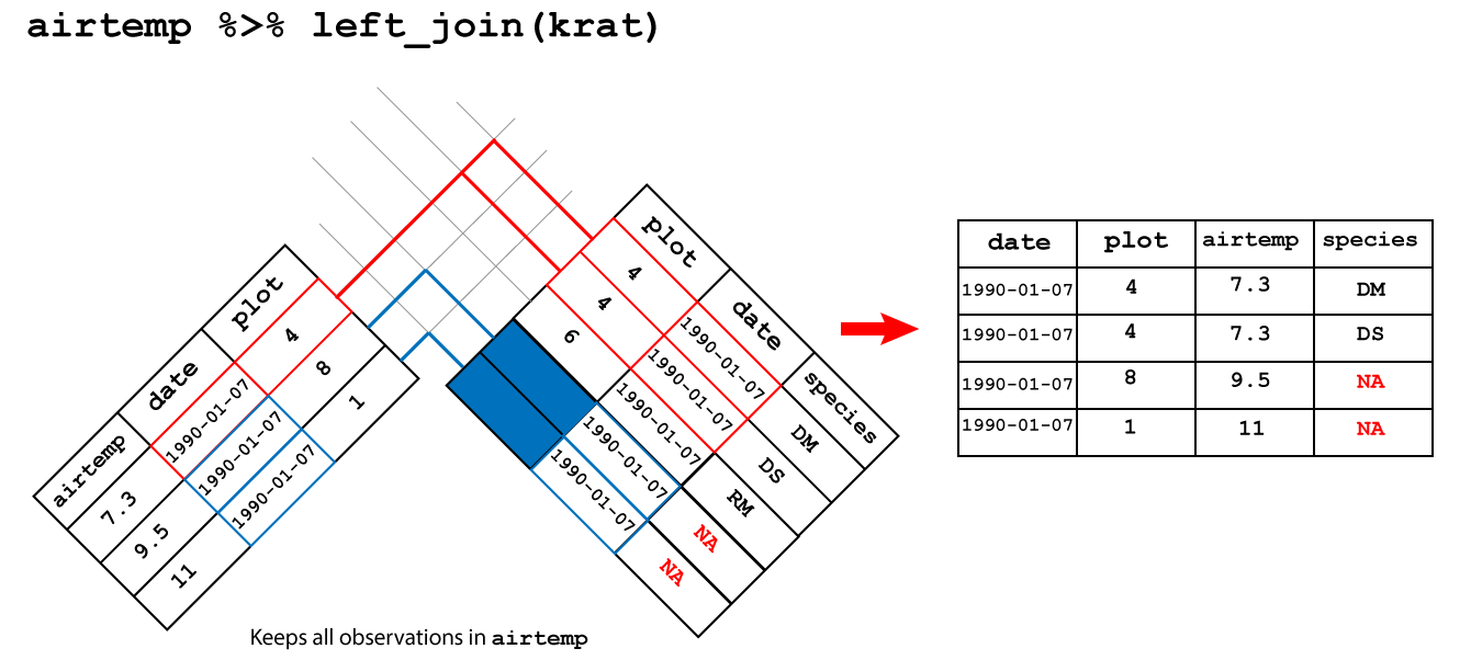
Here, I’ll only cover the join I use the most, left_join(), but there are several joins of each type, which I will leave to you to explore more using the links above.
Let’s say we have a second table which contains the forecast for each day. Here I generate this randomly, but you could equally use readr or readxl to load this data in if you have it in a file.
R
forecast <- weather %>%
  select(date, city) %>%
  mutate(forecast = sample(c("cloudy", "sunny"), size = n(), replace=TRUE))

forecast
OUTPUT
# A tibble: 57 × 3
   date       city   forecast
   <date>     <chr>  <chr>
 1 2022-11-01 sydney cloudy
 2 2022-11-02 sydney sunny
 3 2022-11-03 sydney sunny
 4 2022-11-04 sydney sunny
 5 2022-11-05 sydney cloudy
 6 2022-11-06 sydney sunny
 7 2022-11-07 sydney sunny
 8 2022-11-08 sydney cloudy
 9 2022-11-09 sydney cloudy
10 2022-11-10 sydney cloudy
# … with 47 more rows
Now we would like to join this to our data frame of observations, so we can compare the forecast to what actually happened.
R
weather %>%
  left_join(forecast, by=c("date", "city")) %>%
  select(city, date, sunshine_hours, forecast)
OUTPUT
# A tibble: 57 × 4
   city   date       sunshine_hours forecast
   <chr>  <date>              <dbl> <chr>
 1 sydney 2022-11-01            9.5 cloudy
 2 sydney 2022-11-02           12.8 sunny
 3 sydney 2022-11-03            8.9 sunny
 4 sydney 2022-11-04            5.7 sunny
 5 sydney 2022-11-05           11.8 cloudy
 6 sydney 2022-11-06           12.1 sunny
 7 sydney 2022-11-07           12.3 sunny
 8 sydney 2022-11-08           11   cloudy
 9 sydney 2022-11-09           10.3 cloudy
10 sydney 2022-11-10            9.3 cloudy
# … with 47 more rows
Challenge 7: Blame it on the weatherman
If a cloudy day is one where there are 10 or fewer hours of sunshine, on how many days was the forecast accurate?
R
weather %>%
  # join forecast information
  left_join(forecast, by=c("date", "city")) %>%
  # was forecast accurate
  mutate(forecast_accurate = case_when(
    sunshine_hours > 10 & forecast == "sunny" ~ TRUE,
    sunshine_hours <= 10 & forecast == "cloudy" ~ TRUE,
    TRUE ~ FALSE
  )) %>%
  # count accurate and inaccurate forecasts
  group_by(forecast_accurate) %>%
  summarise(count = n())
OUTPUT
# A tibble: 2 × 2
  forecast_accurate count
  <lgl>             <int>
1 FALSE                28
2 TRUE                 29
Statistical tests
Chances are, you don’t just want to compute means and medians of columns, but actually check if those means or medians are different between groups. For performing statistical tests in R, I have found the rstatix package to be easy to use and well-documented.
For example, if we wanted to do a t-test to check if the maximum temperatures in Brisbane were higher than those in Sydney, we could do:
R
library(rstatix)
OUTPUT
Attaching package: 'rstatix'OUTPUT
The following object is masked from 'package:stats':

    filter
R
weather %>%
  t_test(max_temp_c ~ city,
         alternative="greater")
OUTPUT
# A tibble: 1 × 8
  .y.        group1   group2    n1    n2 statistic    df          p
* <chr>      <chr>    <chr>  <int> <int>     <dbl> <dbl>      <dbl>
1 max_temp_c brisbane sydney    27    28      5.28  43.1 0.00000203
I won’t go into any more detail now, but check out the reference page for the large list of statistical tests that rstatix can perform for you.
Working with large tables
dplyr works well if you have small tables, but when they get large (millions of rows), you might start to notice that your code takes a while to execute. If you start to notice this is an issue (and not before), I’d recommend you check out the dtplyr package](https://dtplyr.tidyverse.org/), which translates dplyr verbs into code used by another, faster package called data.table.
Of course, you could also just learn the data.table package and use it directly, but I find the syntax a little more cryptic than dplyr.
Resources and acknowlegements
- dplyr cheatsheet
- dplyr documentation
- Data transformation in R for data science
- I’ve borrowed figures (and inspiration) from the excellent coding togetheR course material
Keypoints
- Use
summarise()to summarise your data - Use
mutate()to add new columns - Use
filter()to filter rows by a condition - Use
select()to remove or only retain certain rows - Use
arrange()to re-order rows - Use
group_by()to group data by the values in particular columns - Use joins to combine two data frames